Pioneer/Imaging Lab 1
This page serves as a supplement to the first Digital Image Processing Lab for the Summer 2021 Pioneer Program.
Contents
- 1 Corrections / Clarifications to the Handout
- 2 Running Python
- 3 Scikit Image
- 4 Links
- 5 Examples
- 5.1 Example 1: Black & White Images
- 5.2 Example 2: Simple Grayscale Images
- 5.3 Example 3: Less Simple Grayscale Images
- 5.4 Example 4: Building an Image
- 5.5 Example 5: Exploring Colors
- 5.6 Example 6: 1D Convolution
- 5.7 Example 7: 1D Convolution Using "same"
- 5.8 Example 8: 11x11 Blurring
- 5.9 Example 9: Make No Assumptions
- 5.10 Example 10: Basic Edge Detection and Display
- 5.11 Example 11: Chips!
- 5.12 Example 12: Chip Edges!
- 6 Exercise Starter Codes
Corrections / Clarifications to the Handout
- None yet
Running Python
You need to have Anaconda installed, which includes the Spyder IDE and all the modules that we need for this assignment.
Scikit Image
See Pioneer21/Lecture03 for more details about using the scikit-image module.
Links
- 2D Convolution description: HTTP://www.songho.ca/dsp/convolution/convolution2d_example.HTML
- Kernel page on Wikipedia: https://en.wikipedia.org/wiki/Kernel_(image_processing)
- Test Card for Exercise 8: https://en.wikipedia.org/wiki/Test_card
Examples
The following sections will contain both the example programs given in the lab as well as the image or images they produce. You should still type these into your own version of Python to make sure you are getting the same answers. These are provided so you can compare what you get with what we think you should get. All examples and exercises assume you have already run the following code:
import numpy as np
import skimage as ski
import scipy.signal as sig
import matplotlib.pyplot as plt
If there are any other required modules, they will explicitly show up at the top of the example or exercise code.
Example 1: Black & White Images


a = np.array([
    [1, 0, 1, 0, 0],
    [1, 0, 1, 0, 1],
    [1, 1, 1, 0, 0],
    [1, 0, 1, 0, 1],
    [1, 0, 1, 0, 1]])
fig, ax = plt.subplots(num=1, clear=True)
ax.imshow(a, cmap=plt.cm.gray)
ax.set_axis_off()
fig.tight_layout()
fig.savefig("PS21DI1E1Plot1.png")
fig, ax = plt.subplots(num=2, clear=True)
aplot2 = ax.imshow(a, cmap=plt.cm.gray)
fig.colorbar(aplot2)
fig.tight_layout()
fig.savefig("PS21DI1E1Plot2.png")
Example 2: Simple Grayscale Images


bx, by = np.meshgrid(range(255), range(255))
fig, ax = plt.subplots(num=1, clear=True)
aplot1 = ax.imshow(bx, cmap=plt.cm.gray)
fig.colorbar(aplot1)
fig.tight_layout()
fig.savefig("PS21DI1E2Plot1.png")
fig, ax = plt.subplots(num=2, clear=True)
aplot2 = ax.imshow(by, cmap=plt.cm.gray)
fig.colorbar(aplot2)
fig.tight_layout()
fig.savefig("PS21DI1E2Plot1.png")
Example 3: Less Simple Grayscale Images

x, y = np.meshgrid(np.linspace(0, 2*np.pi, 201),
                   np.linspace(0, 2*np.pi, 201));
z = np.cos(x)*np.cos(2*y);
fig, ax = plt.subplots(num=1, clear=True)
zplot = ax.imshow(z, cmap=plt.cm.gray)
ax.axis('equal')
fig.colorbar(zplot)
fig.tight_layout()
fig.savefig("PS21DI1E3Plot1.png")
Notice how the use of ax.axis('equal') made the image look like a square since it is 201x201 but also caused the display to be filled with whitespace as a result of the figure size versus the image size.
Example 4: Building an Image

rad = 100
delta = 10
x, y =np.meshgrid(range((-3*rad-delta),(3*rad+delta)+1),
                  range((-3*rad-delta),(3*rad+delta)+1))
rows, cols = x.shape
dist = lambda x, y, xc, yc: np.sqrt((x-xc)**2+(y-yc)**2)
venn_img = np.zeros((rows, cols, 3));
venn_img[:,:,0] = (dist(x, y, rad*np.cos(0), rad*np.sin(0)) < 2*rad);
venn_img[:,:,1] = (dist(x, y, rad*np.cos(2*np.pi/3), rad*np.sin(2*np.pi/3)) < 2*rad);
venn_img[:,:,2] = (dist(x, y, rad*np.cos(4*np.pi/3), rad*np.sin(4*np.pi/3)) < 2*rad);
fig, ax = plt.subplots(num=1, clear=True)
ax.imshow(venn_img)
ax.axis('equal')
fig.tight_layout()
fig.savefig("PS21DI1E4Plot1.png")
Example 5: Exploring Colors

nr = 256
nc = 256
x, y = np.meshgrid(np.linspace(0, 1, nc),
                   np.linspace(0, 1, nr))
other = 0.5;
palette = np.zeros((nr, nc, 3))
palette[:,:,0] = x
palette[:,:,1] = y
palette[:,:,2] = other
fig, ax = plt.subplots(num=1, clear=True)
ax.imshow(palette)
ax.axis('equal')
fig.tight_layout()
fig.savefig("PS21DI1E5Plot1.png")
Example 6: 1D Convolution
x = np.array([1, 2, 4, 8, 7, 5, -1])
h = np.array([1, -1])
y = sig.convolve(x, h)
print("x: {}\nh: {}\ny: {}".format(x, h, y))
x: [ 1  2  4  8  7  5 -1]
h: [ 1 -1]
y: [ 1  1  2  4 -1 -2 -6  1]
Example 7: 1D Convolution Using "same"
x = np.array([1, 2, 4, 8, 7, 5, -1])
h = np.array([1, -1])
y = sig.convolve(x, h, "same")
print("x: {}\nh: {}\ny: {}".format(x, h, y))
x: [ 1  2  4  8  7  5 -1]
h: [ 1 -1]
y: [ 1  1  2  4 -1 -2 -6]
Example 8: 11x11 Blurring


x = ski.data.coins()
h = np.ones((11, 11))/11**2;
y = sig.convolve2d(x, h, 'same');
fig, ax = plt.subplots(num=1, clear=True)
aplot1 = ax.imshow(x, cmap=plt.cm.gray, vmin=0, vmax=255)
ax.axis('equal')
ax.set(title='Original')
fig.colorbar(aplot1)
fig.tight_layout()
fig.savefig("PS21DI1E8Plot1.png")
fig, ax = plt.subplots(num=2, clear=True)
aplot2 = ax.imshow(y, cmap=plt.cm.gray, vmin=0, vmax=255)
ax.axis('equal')
ax.set(title='Blurred')
fig.colorbar(aplot2)
fig.tight_layout()
fig.savefig("PS21DI1E8Plot2.png")
Example 9: Make No Assumptions
x = np.array([1, 2, 4, 8, 7, 5, -1])
h = np.array([1, -1])
y = sig.convolve(x, h, "valid")
print("x: {}\nh: {}\ny: {}".format(x, h, y))
x: [ 1  2  4  8  7  5 -1]
h: [ 1 -1]
y: [ 1  2  4 -1 -2 -6]
Example 10: Basic Edge Detection and Display
x, y = np.meshgrid(np.linspace(-1, 1, 200),
                   np.linspace(-1, 1, 200));
z1 = (.7<np.sqrt(x**2+y**2)) * (np.sqrt(x**2+y**2)<.9)
z2 = (.3<np.sqrt(x**2+y**2)) * (np.sqrt(x**2+y**2)<.5)
zimg = 100*z1+200*z2;
fig, ax = plt.subplots(num=1, clear=True)
aplot1 = ax.imshow(zimg, cmap=plt.cm.gray, vmin=0, vmax=255)
ax.axis('equal')
ax.set(title='Original')
fig.colorbar(aplot1)
fig.tight_layout()
fig.savefig("PS21DI1E9Plot1.png")

hx = np.array([[1, -1], [1, -1]])
edgex = sig.convolve2d(zimg, hx, 'valid')
fig, ax = plt.subplots(num=2, clear=True)
aplot2 = ax.imshow(edgex, cmap=plt.cm.gray)
ax.axis('equal')
ax.set(title='Vertical Edges')
fig.colorbar(aplot2)
fig.tight_layout()
fig.savefig("PS21DI1E9Plot2.png")

hy = np.array([[1, 1], [-1, -1]])
edgey = sig.convolve2d(zimg, hy, 'valid')
fig, ax = plt.subplots(num=3, clear=True)
aplot3 = ax.imshow(edgey, cmap=plt.cm.gray)
ax.axis('equal')
ax.set(title='Horizontal Edges')
fig.colorbar(aplot3)
fig.tight_layout()
fig.savefig("PS21DI1E9Plot3.png")

edges = np.sqrt(edgex**2 + edgey**2)
fig, ax = plt.subplots(num=4, clear=True)
aplot4 = ax.imshow(edges, cmap=plt.cm.gray)
ax.axis('equal')
ax.set(title='Edges')
fig.colorbar(aplot4)
fig.tight_layout()
fig.savefig("PS21DI1E9Plot4.png")
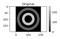
Original
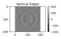
Vertical Edges
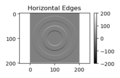
Horizontal Edges
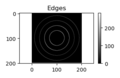
Edges


Example 11: Chips!
For this example, save the image at right to a file called "amandajones_chips_unsplash.jpg" in the same folder as Python is running. This image comes from, Amanda Jones' Unsplash page and is free to use for non-commercial use.

import matplotlib.image as mpimg
from matplotlib.colors import ListedColormap
img = mpimg.imread("amandajones_chips_unsplash.jpg")

fig, ax = plt.subplots(num=1, clear=True)
ax.imshow(img)
ax.axis('equal')
ax.set(title='Original')
fig.tight_layout()
fig.savefig("PS21DI1E11Plot1.png")
vals = np.linspace(0, 1, 256)
names = ['Red', 'Green', 'Blue']
for k in range(3):
    fig, ax = plt.subplots(num=k+2, clear=True)
    aplot1 = ax.imshow(img[:,:,k], cmap=plt.cm.gray, vmin=0, vmax=255)
    ax.axis('equal')
    ax.set(title=names[k]+" as Gray")
    fig.colorbar(aplot1)
    fig.tight_layout()
    fig.savefig("PS21DI1E11Plot{}.png".format(k+2))

    fig, ax = plt.subplots(num=k+5, clear=True)
    mycmvals = np.zeros((256,4))
    mycmvals[:,k] = vals
    mycmvals[:,3] = 1
    mycm = ListedColormap(mycmvals)
    aplot2 = ax.imshow(img[:,:,k], cmap=mycm, vmin=0, vmax=255)
    ax.axis('equal')
    ax.set(title=names[k]+" as "+names[k])
    fig.colorbar(aplot2)
    fig.tight_layout()
    fig.savefig("PS21DI1E11Plot{}.png".format(k+5))
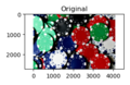
Original

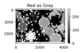
Red as Gray
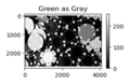
Green as Gray
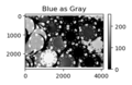
Blue as Gray


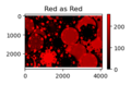
Red as Red
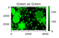
Green as Green
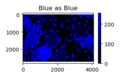
Blue as Blue


Example 12: Chip Edges!
import matplotlib.image as mpimg
imgo = mpimg.imread("amandajones_chips_unsplash.jpg")
img = imgo[::10, ::10, :]

fig, ax = plt.subplots(num=1, clear=True)
ax.imshow(img)
ax.axis('equal')
ax.set(title='Scaled Down Original')
fig.tight_layout()
fig.savefig("PS21DI1E12Plot1.png")
vals = np.linspace(0, 1, 256)
names = ['Red', 'Green', 'Blue']
h = np.array([[1, 0, -1],[ 2, 0, -2], [ 1, 0, -1]])
edgevals = np.zeros((img.shape[0]-h.shape[0]+1,
                     img.shape[1]-h.shape[1]+1,
                     3))
for k in range(3):
    fig, ax = plt.subplots(num=k+2, clear=True)
    edgevals[:,:,k] = sig.convolve2d(img[:,:,k], h, "valid")
    aplot1 = ax.imshow(edgevals[:,:,k], cmap=plt.cm.gray, vmin=-1020, vmax=1020)
    ax.axis('equal')
    ax.set(title=names[k]+" Edges as Gray")
    fig.colorbar(aplot1)
    fig.tight_layout()
    fig.savefig("PS21DI1E12Plot{}.png".format(k+2))

    fig, ax = plt.subplots(num=k+5, clear=True)
    aplot2 = ax.imshow(edgevals[:,:,k], cmap=plt.cm.gray, vmin=0, vmax=1020)
    ax.axis('equal')
    ax.set(title="Absolute " + names[k]+" Edges as Gray")
    fig.colorbar(aplot2)
    fig.tight_layout()
    fig.savefig("PS21DI1E12Plot{}.png".format(k+5))

fig, ax = plt.subplots(num=8, clear=True)
edgevals2 = (edgevals + abs(edgevals).max()) / 2 / abs(edgevals).max()
ax.imshow(edgevals2)
ax.axis('equal')
ax.set(title="Colorful Edges")
fig.tight_layout()
fig.savefig("PS21DI1E12Plot8.png")

fig, ax = plt.subplots(num=9, clear=True)
edgevals3 = np.linalg.norm(edgevals, ord=2, axis=2)
ax.imshow(edgevals3, cmap=plt.cm.gray)
ax.axis('equal')
ax.set(title="Absolute Edges")
fig.tight_layout()
fig.savefig("PS21DI1E12Plot9.png")
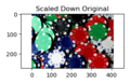
Original

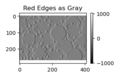
Red Edges as Gray
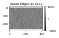
Green Edges as Gray

Blue Edges as Gray


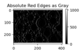
Absolute Red Edges as Gray
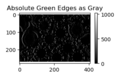
Absolute Green Edges as Gray

Absolute Blue Edges as Gray


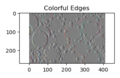
Colorful Edges
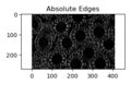
Absolute Edges


Exercise Starter Codes
Exercise 3
tc = np.linspace(0, 1, 101)
td = np.linspace(0, 1, 11)
myfun = lambda x: np.sin(20*x)*np.exp(-2*x)
xc = myfun(tc)
xd = myfun(td)
fig, ax = plt.subplots(num=1, clear=True)
ax.plot(tc, xc, 'b-')
ax.plot(td, xd, 'bo')
Exercise 4
tc = np.linspace(0, 1, 101)
td = np.linspace(0, 1, 11)
deltatc = tc[1]-tc[0]
deltatd = td[1]-td[0]

myfun = lambda x: np.sin(20*x)*np.exp(-2*x)
xc = myfun(tc)
xd = myfun(td)

fig, ax = plt.subplots(num=1, clear=True)
ax.plot(tc, xc, 'b-')
ax.plot(td, xd, 'bo')
ax.set(title='Values')
fig.tight_layout()

fig, ax = plt.subplots(num=2, clear=True)
twopointdiff = np.diff(xc)/deltatc
twopointdiff = np.append(twopointdiff, twopointdiff[-1])
ax.plot(tc, twopointdiff, 'b-')
ax.plot(tc[::10], twopointdiff[::10], 'bo')
ax.set(title='Change Me')
fig.tight_layout()