EGR 103/Concept List Fall 2019
This page will be used to keep track of the commands and major concepts for each lecture in EGR 103.
Contents
- 1 Lecture 1 - Introduction
- 2 Lecture 2 - Programs and Programming
- 3 Lecture 3 - "Number" Types
- 4 Lecture 4 - Other Types and Functions
- 5 Lecture 5 - Format, Logic, Decisions, and Loops
- 6 Lecture 6 - String Things and Loops
- 7 Lecture 7 - Applications
- 8 Lecture 8 - Taylor Series and Iterative Solutions
- 9 Lecture 9 - Binary and Floating Point Numbers
- 10 Lecture 10 - Monte Carlo Methods
- 11 Lecture 11 - Style, Code Formatters, Docstrings, and More Walking
- 12 Lecture 12 - Arrays and Matrix Representation in Python
- 13 Lecture 13 - Linear Algebra and Solutions
- 14 Lecture 14 - Solution Sweeps, Norms, and Condition Numbers
- 15 Lecture 15
- 16 Lecture 16
- 17 Lecture 17 - Statistics and Curve Fits
- 18 Lecture 18 - More statistics and curve fitting
- 19 Lecture 19 - 3D Plotting
- 20 Lecture 20 - Roots of Equations
- 21 Lecture 21 - Roots and Extrema
- 22 Lecture 22 - Interpolation
- 23 Lecture 23 - Numerical Differentiation and Integration
- 24 Lecture 24 - Test Review
Lecture 1 - Introduction
- Class web page: EGR 103L; assignments, contact info, readings, etc - see slides on Errata/Notes page
- Sakai page: Sakai 103L page; grades, surveys and tests, some assignment submissions
- CampusWire page: CampusWire 103L page; message board for questions - you need to be in the class and have the access code to subscribe.
Lecture 2 - Programs and Programming
- Seven steps of programming -
- Watch video on Developing an Algorithm
- Watch video on A Seven Step Approach to Solving Programming Problems
- To play with Python:
- Install it on your machine or a public machine: Download
- Quick tour of Python
- Editing window, variable explorer, and console
- You are not expected to remember any of the specifics about how Python stores things or works with them yet!
Lecture 3 - "Number" Types
- Python is a "typed" language - variables have types
- We will use eight types:
- Focus of the day: int, float, and array
- Focus a little later: string, list, tuple
- Focus later: dictionary, set
- int: integers; Python can store these perfectly
- float: floating point numbers - "numbers with decimal points" - Python sometimes has problems
- array
- Requires numpy, usually with
import numpy as np - Organizational unit for storing rectangular arrays of numbers
- Requires numpy, usually with
- Math with "Number" types works the way you expect
- ** * / // % + -
- Relational operators can compare "Number" Types and work the way you expect with True or False as an answer
- < <= == >= > !=
- With arrays, either same size or one is a single value; result will be an array of True and False the same size as the array
- Slices allow us to extract information from an array or put information into an array
- a[0] is the element in a at the start
- a[3] is the element in a three away from the start
- a[:] is all the elements in a because what is really happening is:
- a[start:until] where start is the first index and until is just *past* the last index;
- a[3:7] will return a[3] through a[6] in 4-element array
- a[start:until:increment] will skip indices by increment instead of 1
- To go backwards, a[start:until:-increment] will start at an index and then go backwards until getting at or just past until.
- For 2-D arrays, you can index items with either separate row and column indices or indices separated by commas:
- a[2][3] is the same as a[2, 3]
- Only works for arrays!
Lecture 4 - Other Types and Functions
- Lists are set off with [ ] and entries can be any valid type (including other lists!); entries can be of different types from other entries
- List items can be changed
- Tuples are indicated by commas without square brackets (and are usually shown with parentheses - which are required if trying to make a tuple an entry in a tuple or a list)
- Dictionaries are collections of key : value pairs set off with { }; keys can be any immutable type (int, float, string, tuple) and must be unique; values can be any type and do not need to be unique
- To read more:
- Note! Many of the tutorials below use Python 2 so instead of
print(thing)it showsprint thing - Lists at tutorialspoint
- Tuples at tutorialspoint
- Dictionary at tutorialspoint
- Note! Many of the tutorials below use Python 2 so instead of
- Defined functions can be multiple lines of code and have multiple outputs.
- Four different types of input parameters:
- Required (listed first)
- Named with defaults (second)
- Additional positional arguments ("*args") (third)
- Function will create a tuple containing these items in order
- Additional keyword arguments ("**kwargs") (last)
- Function will create a dictionary of keyword and value pairs
- Function ends when indentation stops or when the function hits a return statement
- Return returns single item as an item of that type; if there are multiple items returned, they are stored in a tuple
- If there is a left side to the function call, it either needs to be a single variable name or a tuple with as many entries as the number of items returned
- Four different types of input parameters:
Lecture 5 - Format, Logic, Decisions, and Loops
- Creating formatted strings using {} and .format() (format strings, standard format specifiers) -- focus was on using e or f for type, minimumwidth.precision, and possibly a + in front to force printing + for positive numbers.
- Also - Format Specification Mini-Language
- Basics of decisions using if...elif...else
- Building a program to check for vowels, consonants, and y
- Bonus material:
- Rhabarberbarbara - now with subtitles!
- Rhabarberbarbara - live recording!
- Lion-Eating Poet in the Stone Den - 施氏食獅史, or Shī Shì shí shī shǐ
- Buffalo$$^8$$
Lecture 6 - String Things and Loops
ordto get numerical value of each characterchrto get character based on integermap(fun, sequence)to apply a function to each item in a sequence- Basics of while loops
- Basics of for loops
- List comprehensions
- [FUNCTION for VAR in SEQUENCE if LOGIC]
- The FUNCTION should return a single thing (though that thing can be a list, tuple, etc)
- The "if LOGIC" part is optional
[k for k in range(3)]creates[0, 1, 2][k**2 for k in range (5, 8)]creates[25, 36, 49][k for k in 'hello' if k<'i']creates['h', 'e'][(k,k**2) for k in range(11) if k%3==2]creates[(2, 4), (5, 25), (8, 64)]
- [FUNCTION for VAR in SEQUENCE if LOGIC]

- Wait - that's the simplified version...here:
- Wait - that's the simplified version...here:
- Want to see Amharic?

list(map(chr, range(4608, 4992)))
- Want to see the Greek alphabet?
for k in range(913,913+25):
    print(chr(k), chr(k+32))
Lecture 7 - Applications
- The Price Is Right - Clock Game video demonstration
# tpir.py from class:
import numpy as np
import time

def create_price(low=100, high=1500):
    return np.random.randint(low, high+1)

def get_guess():
    guess = int(input('Guess: '))
    return guess

def check_guess(actual, guess):
    if actual > guess:
        print('Higher!')
    elif actual < guess:
        print('Lower!')


if __name__ == '__main__':
    #print(create_price(0, 100))
    the_price = create_price()
    the_guess = get_guess()
    start_time = time.clock()
    #print(the_guess)
    while the_price != the_guess and (time.clock() < start_time+30):
        check_guess(the_price, the_guess)
        the_guess = get_guess()

    if the_price==the_guess:
        print('You win!!!!!!!')
    else:
        print('LOOOOOOOOOOOOOOOSER')
- NATO Phonetic Translator - NATO phonetic alphabet
# nato_trans.py from class:
fread = open('NATO.dat', 'r')

d = {}

for puppies in fread:
    #print(puppies) $ if you want to see the whole line

    #key = puppies[0]
    #value = puppies[:-1]
    #d[key] = value

    d[puppies[0]] = puppies[:-1]

fread.close()

hamster = input('Word: ').upper()

for kittens in hamster:
    #print(d[letter], end=' ')
    print(d.get(kittens, 'XXX'), end=' ')

'''
In class - one question was "in cases where there is not a code, can it
return the original value instead of XXX" -- yes:
    print(d.get(kittens, kittens))
'''
- Data file we used:
# NATO.dat from class:
Alfa
Bravo
Charlie
Delta
Echo
Foxtrot
Golf
Hotel
India
Juliett
Kilo
Lima
Mike
November
Oscar
Papa
Quebec
Romeo
Sierra
Tango
Uniform
Victor
Whiskey
X-ray
Yankee
Zulu
Lecture 8 - Taylor Series and Iterative Solutions
- Taylor series fundamentals
- Maclaurin series approximation for exponential uses Chapra 4.2 to compute terms in an infinite sum.
- so
- Newton Method for finding square roots uses Chapra 4.2 to iteratively solve using a mathematical map. To find \(y\) where \(y=\sqrt{x}\):
\( \begin{align} y_{init}&=1\\ y_{new}&=\frac{y_{old}+\frac{x}{y_{old}}}{2} \end{align} \) - See Python version of Fig. 4.2 and modified version of 4.2 in the Resources section of Sakai page under Chapra Pythonified
Lecture 9 - Binary and Floating Point Numbers
- Different number systems convey information in different ways.
- Roman Numerals
- Chinese Numbers
- Ndebe Igbo Numbers
- Binary Numbers
- We went through how to convert between decimal and binary
- Kibibytes et al
- "One billion dollars!" may not mean the same thing to different people: Long and Short Scales
- Floats (specifically double precision floats) are stored with a sign bit, 52 fractional bits, and 11 exponent bits. The exponent bits form a code:
- 0 (or 00000000000): the number is either 0 or a denormal
- 2047 (or 11111111111): the number is either infinite or not-a-number
- Others: the power of 2 for scientific notation is 2**(code-1023)
- The largest number is thus just *under* 2**1024 (ends up being (2-2**-52)**1024\(\approx 1.798\times 10^{308}\).
- The smallest normal number (full precision) is 2**(-1022)\(\approx 2.225\times 10^{-308}\).
- The smallest denormal number (only one significant binary digit) is 2**(-1022)/2**53 or 5e-324.
- When adding or subtracting, Python can only operate on the common significant digits - meaning the smaller number will lose precision.
- (1+1e-16)-1=0 and (1+1e-15)-1=1.1102230246251565e-15
- Avoid intermediate calculations that cause problems: if x=1.7e308,
- (x+x)/x is inf
- x/x + x/x is 2.0
- In cases where mathematical formulas have limits to infinity, you have to pick numbers large enough to properly calculate values but not so large as to cause errors in computing:
- $$e^x=\lim_{n\rightarrow \infty}\left(1+\frac{x}{n}\right)^n$$
# Exponential Demo
<syntaxhighlightlang=python> import numpy as np import matplotlib.pyplot as plt
def exp_calc(x, n):
return (1 + x/n)**n
if __name__ == "__main__":
   n = np.logspace(0, 17, 1000)
   y = exp_calc(1, n)
   fig, ax = plt.subplots(num=1, clear=True)
   ax.semilogx(n, y)
   fig.savefig('ExpDemoPlot1.png')

   # Focus on right part
   n = np.logspace(13, 16, 1000)
   y = exp_calc(1, n)
   fig, ax = plt.subplots(num=2, clear=True)
   ax.semilogx(n, y)
   fig.savefig('ExpDemoPlot2.png')
</syntaxhighlight>
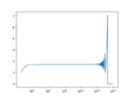
estimates for calculating $$e$$ with $$n$$ between 1 and $$1*10^{17}$$
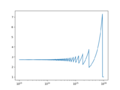
$$n$$ between $$10^{13}$$ and $$10^{16}$$ showing region when roundoff causes problems


Lecture 10 - Monte Carlo Methods
- See walk1 in Resources section of Sakai
Lecture 11 - Style, Code Formatters, Docstrings, and More Walking
- Discussion of PEP and PEP8 in particular
- Autostylers include black, autopep8, and yapf -- we will mainly use black
- To get the package:
- On Windows start an Anaconda Prompt (Start->Anaconda3->Anaconda Prompt) or on macOS open a terminal and change to the \users\name\Anaconda3 folder
pip install blackshould install the code
- To use that package:
- Change to the directory where you files lives. On Windows, to change drives, type the driver letter and a colon by itself on a line, then use cd and a path to change directories; on macOS, type
cd /Volumes/NetIDwhere NetID is your NetID to change into your mounted drive. - Type
black FILE.pyand note that this will actually change the file - be sure to save any changes you made to the file before runningblack - As noted in class, black automatically assumes 88 characters in a line; to get it to use the standard 80, use the
-l 80adverb, e.g.black FILE.py -l 80
- Change to the directory where you files lives. On Windows, to change drives, type the driver letter and a colon by itself on a line, then use cd and a path to change directories; on macOS, type
- To get the package:
- Docstrings
- We will be using the numpy style at docstring guide
- Generally need a one-line summary, summary paragraph (if needed), a list of parameters, and a list of returns
- Specific formatting chosen to allow Spyder's built in help tab to format file in a pleasing way
- More walking
- We went through the walk_1 code again and then decided on three different ways we could expand it and looked at how that might impact the code:
- Choose from more integers than just 1 and -1 for the step: very minor impact on code
- Choose from a selection of floating point values: minor impact other than a bit of documentation since ints and floats operate in similar ways
- Walk in 2D rather than along a line: major impact in terms of needing to return x and y value for the step, store x and y value for the location, plot things differently
- All codes from today will be on Sakai in Resources folder
Lecture 12 - Arrays and Matrix Representation in Python
- 1-D and 2-D Arrays
- Python does mathematical operations differently for 1 and 2-D arrays
- Matrix multiplication (by hand)
- Matrix multiplication (using @ in Python)
- To multiply matrices A and B ($$C=A\times B$$ in math or
C=A@Bin Python) using matrix multiplication, the number of columns of A must match the number of rows of B; the results will have the same number of rows as A and the same number of columns as B. Order is important - Setting up linear algebra equations
- Determinants of matrices and the meaning when the determinant is 0
- Shortcuts for determinants of 1x1, 2x2 and 3x3 matrices (see class notes for processes)
- $$\begin{align*} \mbox{det}([a])&=a\\ \mbox{det}\left(\begin{bmatrix}a&b\\c&d\end{bmatrix}\right)&=ad-bc\\ \mbox{det}\left(\begin{bmatrix}a&b&c\\d&e&f\\g&h&i\end{bmatrix}\right)&=aei+bfg+cdh-afh-bdi-ceg\\ \end{align*}$$
- Don't believe me? Ask Captain Matrix!
Lecture 13 - Linear Algebra and Solutions
- Inverses of matrices:
- Generally, $$\mbox{inv}(A)=\frac{\mbox{cof}(A)^T}{\mbox{det}(A)}$$ there the superscript T means transpose...
- And $$\mbox{det}(A)=\sum_{i\mbox{ or }j=0}^{N-1}a_{ij}(-1)^{i+j}M_{ij}$$ for some $$j$$ or $$i$$...
- And $$M_{ij}$$ is a minor of $$A$$, specifically the determinant of the matrix that remains if you remove the $$i$$th row and $$j$$th column or, if $$A$$ is a 1x1 matrix, 1
- And $$\mbox{cof(A)}$$ is a matrix where the $$i,j$$ entry $$c_{ij}=(-1)^{i+j}M_{ij}$$
- And $$M_{ij}$$ is a minor of $$A$$, specifically the determinant of the matrix that remains if you remove the $$i$$th row and $$j$$th column or, if $$A$$ is a 1x1 matrix, 1
- And $$\mbox{det}(A)=\sum_{i\mbox{ or }j=0}^{N-1}a_{ij}(-1)^{i+j}M_{ij}$$ for some $$j$$ or $$i$$...
- Good news - for this class, you need to know how to calculate inverses of 1x1 and 2x2 matrices only:
- Generally, $$\mbox{inv}(A)=\frac{\mbox{cof}(A)^T}{\mbox{det}(A)}$$ there the superscript T means transpose...
- $$ \begin{align} \mbox{inv}([a])&=\frac{1}{a}\\ \mbox{inv}\left(\begin{bmatrix}a&b\\c&d\end{bmatrix}\right)&=\frac{\begin{bmatrix}d &-b\\-c &a\end{bmatrix}}{ad-bc} \end{align}$$
- Converting equations to a matrix system:
- For a certain circuit, conservation equations learned in upper level classes will yield the following two equations:
- $$\begin{align} \frac{v_1-v_s}{R1}+\frac{v_1}{R_2}+\frac{v_1-v_2}{R_3}&=0\\ \frac{v_2-v_1}{R_3}+\frac{v_2}{R_4}=0 \end{align}$$
- Assuming $$v_s$$ and the $$R_k$$ values are known, to write this as a matrix equation, you need to get $$v_1$$ and $$v_2$$ on the left and everything else on the right:
- $$\begin{align} \left(\frac{1}{R_1}+\frac{1}{R_2}+\frac{1}{R_3}\right)v_1+\left(-\frac{1}{R_3}\right)v_2&=\frac{v_s}{R_1}\\ \left(-\frac{1}{R_3}\right)v_1+\left(\frac{1}{R_3}+\frac{1}{R_4}\right)v_2&=0 \end{align}$$
- Now you can write this as a matrix equation:
$$ \newcommand{\hmatch}{\vphantom{\frac{1_s}{R_1}}} \begin{align} \begin{bmatrix} \frac{1}{R_1}+\frac{1}{R_2}+\frac{1}{R_3} & -\frac{1}{R_3} \\ -\frac{1}{R_3} & \frac{1}{R_3}+\frac{1}{R_4} \end{bmatrix} \begin{bmatrix} \hmatch v_1 \\ \hmatch v_2 \end{bmatrix} &= \begin{bmatrix} \frac{v_s}{R_1} \\ 0 \end{bmatrix} \end{align}$$
Lecture 14 - Solution Sweeps, Norms, and Condition Numbers
- See Python:Linear_Algebra#Sweeping_a_Parameter for example code on solving a system of equations when one parameter (either in the coefficient matrix or in the forcing vector or potentially both)
- Chapra 11.2.1 for norms
- np.linalg.nrom() in Python
- Chapra 1.2.2 for condition numbers
- np.linalg.cond() in Python
- Note: base-10 logarithm of condition number gives number of digits of precision possibly lost due to system geometry and scaling (top of p. 295 in Chapra)
Lecture 15
- Test Review
Lecture 16
- Test
Lecture 17 - Statistics and Curve Fits
- Definition of curve fitting versus interpolation:
- Curve fitting involves taking a scientifically vetted model, finding the best coefficients, and making predictions based on the model. The model may not perfectly hit any of the actual data points.
- Interpolation involves making a guess for values between data points. Interpolants actually hit all the data points but may have no scientific validity at all. Interpolation is basically "connecting the dots," which may involve mathematically complex formulae.
- Statistical definitions used (see Statistics Symbols for full list):
- $$x$$ will be used for independent data
- $$y$$ will be used for dependent data
- $$\bar{x}$$ and $$\bar{y}$$ will be used for the averages of the $$x$$ and $$y$$ sets
- $$\hat{y}_k$$ will be used for the estimate of the $$k$$th dependent point
- $$S_t=\sum_k\left(y_k-\bar{y}\right)^2$$ is the sum of the squares of the data residuals and gives a measure of the spread of the data though any given value can mean several different things for a data set. It will be a non-negative number; a value of 0 implies all the $$y$$ values are the same.
- $$S_r=\sum_k\left(y_k-\hat{y}_k\right)^2$$ is the sum of the squares of the squares of the estimate residuals and gives a measure of the colletive distance between the data points and the model equation for the data points. It will be a non-negative number; a value of 0 implies all the estimates are mathematically perfectly predicted by the model.
- $$r^2=\frac{S_t-S_r}{S_t}=1-\frac{S_r}{S_t}$$ is the coefficient of determination; it is a normalized value that gives information about how well a model predicts the data. An $$r^2$$ value of 1 means the model perfectly predicted every value in the data set. A value of 0 means the model does as well as having picked the average. A negative value means the model is worse than merely picking the average.
Lecture 18 - More statistics and curve fitting
- Mathematical proof of solution to General Linear Regression
- Python:Fitting
Lecture 19 - 3D Plotting
Lecture 20 - Roots of Equations
- Python:Finding roots
- SciPy references (all from Optimization and root finding):
- scipy.optimize.brentq - closed method root finding
- scipy.optimize.fsolve - open method root finding
Lecture 21 - Roots and Extrema
- Python:Extrema
- SciPy references (all from Optimization and root finding):
- scipy.optimize.fmin - unbounded minimization
- scipy.optimize.fminbound - bounded minimization
Lecture 22 - Interpolation
- Python:Interpolation
- Interpolation is a process by which you can "fill in the gaps" of a data set.
- Unlike a model, the functions used to interpolate may have no scientific validity; instead, they satisfy different mathematical conditions.
- The main interpolations we looked at are nearest neighbor, linear, and cubic spline with different conditions (not-a-knot, clamped, natural)
Lecture 23 - Numerical Differentiation and Integration
- Estimates for derivatives and integrals come from deciding which interpolation to work with and using that to either find slopes or integrals.
Lecture 24 - Test Review
This was going to be all about ODEs. It wasn't.