EGR 103/Concept List/F23
Jump to navigation
Jump to search
\(
y=e^x=\sum_{n=0}^{\infty}\frac{x^n}{n!}
\)
\(
\begin{align}
y_{init}&=1\\
y_{new}&=y_{old}+\frac{x^n}{n!}
\end{align}
\)
Contents
- 1 Lecture 1 - 8/28 - Course introduction
- 2 Lecture 2 - 9/1 - Introduction to programming
- 3 Lecture 3 - 9/4 - Introduction to Python
- 4 Lecture 4 - 9/8 - Built-in functions, formatted printing
- 5 Lecture 5 - 9/11 - Intro to lists, tuples, and strings; Intro to graphs
- 6 Lecture 6 - 9/15 - Intro to functions
- 7 Lecture 7 - 9/18 - Functions continued; Decisions
- 8 Lecture 8 - 9/22 - Loops
- 9 Lecture 9 - 9/25 - More Strings and Dictionaries
- 10 Lecture 10 - 9/29 - Surfaces
- 11 Lecture 11 - 10/2 - Coordinate Systems
- 12 Lecture 12 - 10/6 - Numerical Representation and Unavoidable Errors
- 13 Lecture 13 - 10/9 - Iterative Methods for Maps and Accumulations
- 14 Lecture 14 - 10/13 - Logical Masks
- 15 Lecture 15 - 10/15 - Monte Carlo Methods
- 16 Lecture 16 - 10/23 - Roots
- 17 Lecture 17 - 10/27 - More Roots
- 18 Lecture 18 - 10/30 - Optimization
- 19 Lecture 19 - 11/3 - Complex Number intro; Newton Fractals
- 20 Lecture 20 - 11/6 - Basic Linear Algebra
- 21 Lecture 21 - 11/10 - Numerical Integration
- 22 Lecture 22 - 11/13 - Numerical Differentiation
- 23 Lecture 23 - 11/17 - Object-oriented Programming
- 24 Lecture 24 - 11/20 - More Object-oriented Programming
- 25 Lecture 25 - 11/27 - Curve Fitting
- 26 Lecture 27 - 12/4 - More Initial Value Problems
- 27 Lecture 28 - 12/8 - Demos
Lecture 1 - 8/28 - Course introduction
- Main class page: EGR 103L
- Includes links to Canvas, Pundit, and Ed pages
- Sakai page: Canvas103L page; grades, surveys and tests, some assignment submissions; first day slideshow in Resources section goes over everything else.
- For next Friday's class:
- Log in at Coursera at Duke
- Watch video on Developing an Algorithm
- Watch video on A Seven Step Approach to Solving Programming Problems
- See Seven steps of programming The Seven Steps Poster.
Lecture 2 - 9/1 - Introduction to programming
- Seven steps of programming The Seven Steps Poster
- Watch video on Developing an Algorithm
- Watch video on A Seven Step Approach to Solving Programming Problems
- Almost all languages have input, output, math, conditional execution (decisions), and repetition (loops)
- Problem: Consider how to decide if a number is a prime number
- Some "shortcuts" for specific factors (2, 3, and 5, for example) but need to have a generalized approach
- See if number is evenly divisible by any integer between 2 and the square root of the number - but how do we ask the computer to do that?
- We can use output to get the computer to ask for a number and we can use input to allow the computer to receive that number
- We can use math and the mod operator (%) to see if one number is evenly divisible by another, a loop to go through all possible relevant divisors, and a decision structure to choose what to do if we determine that a number is not prime.
- Very quick tour of Python with Spyder
- Console (with history tab), info box (with variable explorer, files, and other tabs), and editing window
- Pushing "play" button or hitting F5 will save the script, change the working directory, and run the script
- Quick introduction to variable types: int, float, str
- Quick introduction to indexing: Python is "0" indexed, meaning if there is a collection of items called x, x[0] will be the "first" item in the collection and x[N-1] where N is the total number of items will be the last item. Also, reverse indexing, where x[-1] is the last item and x[-N] is the first item.
Lecture 3 - 9/4 - Introduction to Python
- No lecture due to Labor Day
- See User:DukeEgr93/ld for a summary of work to do instead!
Lecture 4 - 9/8 - Built-in functions, formatted printing
- Python doesn't know everything to start with; may need to import things
import MODULEmeans usingMODULE.function()to run - brings in everything in the module under the module's nameimport MODULE as NAMEmeans usingNAME.function()to run - this is the most common one for usfrom MODULE import FUNCTION1, FUNCTION2, ...means using FUNCTION1(), FUNCTION2() as function calls - be careful not to override thingsfrom MODULE import *means importing every function and constant from a module into their own name - very dangerous!
- Arrays
- Must import numpy for arrays
import numpy as npwill be a very common part of code for EGR 103- Organizational unit for storing rectangular arrays of numbers
- Generally create with np.array(LIST) where depth of nested LIST is dimensionality of array
- np.array([1, 2, 3]) is a 1-dimensional array with 3 elements
- np.array([[1, 2, 3], [4, 5, 6]]) is a 2-dimension array with 2 rows and 3 columns
- Math with arrays works the way you expect
- ** * / // % + -
- With arrays, * and / work element by element; *matrix* multiplication is a different character (specifically, @)
- ** * / // % + -
- Creating formatted strings using {} and .format() (format strings, standard format specifiers) -- focus was on using s for string and e or f for numerical types, minimumwidth.precision, and possibly a + in front to force printing + for positive numbers.
- Using {} by themselves will substitute items in order from the
format()function into the string that gets created - Putting a number in the {} will tell
formatwhich thing to get - Format specification comes after a : in the {}; if you do not specify a location index, you still have to put a colon in the {}
- {:s} means string and {:Xs} where X is an integer means reserve at least that much space for a left-formatted string; {:>s} or {:>Xs} where X is a number will right-justify the string
- {:f} means floating point (default 6 digits after decimal point) and {:X.Yf} reserves at least X spaces (including + or - and the . if it is there) with Y digits after the decimal point for t right-justified number
- {:e} means floating point (default 6 digits after decimal point) and {:X.Ye} reserves at least X spaces (including + or - and the . if it is there and the letter e and the + or - after the e and the two or three digit number after that) with Y digits after the decimal point for t right-justified number
- Aside - Format Specification Mini-Language has all the possibilities; we will cover some but not all of these in later classes
- You can enter numbers in scientific notation with a number followed by the letter
eand then a number or negative number for the power of 10; for example,x = 6.02e23ore = -1.6e-19 - float can convert scientific notation as well:
float("1e-5")
- Using {} by themselves will substitute items in order from the
Lecture 5 - 9/11 - Intro to lists, tuples, and strings; Intro to graphs
- Lists are set off with [ ] and entries can be any valid type (including other lists!); entries can be of different types from other entries; list items can be changed and mutable items within lists can be changed. Lists can be "grown" by using += with the list or l.append().
- Tuples are indicated by commas without square brackets (and are usually shown with parentheses - which are required if trying to make a tuple an entry in a tuple or a list); tuple items cannot be changed but mutable items within tuples can be
- Strings are set off with " " or ' ' and contain characters; string items cannot be changed
- For lists, tuples, and strings:
- Using + concatenates the two collections
- Using * with them creates a collection with the original repeated that many times
- Using += will create a new item with something appended to the old item; the "something" needs to be the same type (list, tuple, or string); this may seem to break the "can't be changed" rule but really
a += bisa = a + bwhich creates a newa.
- Trinket
- To read more:
- Plotting
- Need to import matplotlib.pyplot as plt
- Create a figure, cerate a set of axes within the figure, plot using that set of axes
- Plots can have different colors, line styles, and/or point styles
- Labels and title are added with the set command
- See Python:Plotting for more info
Lecture 6 - 9/15 - Intro to functions
- Defined functions can be multiple lines of code and have multiple outputs - we looked at a single output.
 def FNAME(local1, local2, ...):
     CODE
     return THING
- Four different types of input parameters - we only really talked about the first two kinds:
- Required (listed first)
- Named with defaults (second)
- We will cover the other kinds later
- Additional positional arguments ("*args") (third)
- Additional keyword arguments ("**kwargs") (last)
- Function ends when indentation stops or when the function hits a return statement
- Return returns single item as an item of that type
- The function can see things in the console but the console can't see things in the function
- When calling the function, you can put arguments in the order the function expects them to appear or you can give the local names when you call the function. You can do some of both, but the "in order" arguments have to be first; once you name one argument in a function call you *must* name all the rest.
- Four different types of input parameters - we only really talked about the first two kinds:
- Writing test codes
- You will usually test functions by running a script with the function in it; autograders will generally test code by importing the function from your script.
- Python has a default variable called
__name__that tells you who is running the show - it will be"__main__"if you run a script from the console and it will be the same as the name of the file if you are importing from that file. - Given that, including the line
if __name__=="__main__":before test code means the test code will run if you run the script with F5 or the play button but not run if you import the function from the module.
Lecture 7 - 9/18 - Functions continued; Decisions
- Defined functions can be multiple lines of code and have multiple outputs - now lets talk multiple outputs!
 def FNAME(local1, local2, ...):
     CODE
     return THING1, THING 2
- If there are multiple items returned, they are stored and returned in a tuple
- If there is a left side to the function call, it either needs to be a single variable name or a tuple with as many entries as the number of items returned
- <= < == >= > != work with many types; just be careful about interpreting
notcan reverse whileandandorcan combine logical expressions- Basics of decisions using if...elif...else
- Must have logic after if
- Can have as many elif with logic after
- Can have an else without logic at the end
- Flow is solely dependent on indentation!
- Branches can contain other trees for follow-up questions
Lecture 8 - 9/22 - Loops
- Basics of loops using while
- Must have logic; gets evaluated at start and not again until branch ends
- Useful when you do not know how many times a loop will run (input validation example)
- break in a loop can break out early
- continue in a loop goes back to the top early
- Basics of loops using for
- for VAR in ITERABLE
- VAR will take on each item in ITERABLE one at a time; ITERABLE can be a string, list, tuple, array, or range
- range(N) creates something similar to [0, 1, 2, 3, 4, ..., N-1]
- range(M, N) creates something similar to [M, M+1, M+2, ..., N-1]
- range only creates integers
- VAR will take on each item in ITERABLE one at a time; ITERABLE can be a string, list, tuple, array, or range
- Many ways to keep track of items
- Loop over indices and access specific item in iterable
- Loop over iterable and keep a separate counter variable
- Use
enumerate(iterable)to create an iterable made up of tuples where the index is entry 0 and the item is entry 1
- for VAR in ITERABLE
Lecture 9 - 9/25 - More Strings and Dictionaries
- Strings
- Iterable, so you can use a for loop to go through individual letters
- for idx, letter in enumerate(the_string): could be handy
- the_string.split("something") will create a list of strings based on splitting the_string at "something" - usually a space with " "
- "glue".join(a_list) will take strings that are elements in the list and put them into a single string separated by the glue
- ord(char) will give the numerical value of that character; chr(num) will give the character at number num
- Dictionaries
- Collections whose indices are immutables (integer, float, string, tuple)
- Built with d={key1:values, key2:value2}
- Extended with d[newkey]=newvalue
- Look up values with d[key] or d.get(key) or d.get(key, other); for the latter two, if key is not in the dictionary, the get version will return None or other if other is an option.
- d.keys() will give the keys, d.value() will give the values, and d.items() will give tuples containing the key and the values - the latter is very useful for making a loop using for idx, val in d.items():
Lecture 10 - 9/29 - Surfaces
- Various ways to set up 3D space on 2D media; Python has $$x$$ coming towards you and to the right, $$y$$ going away from you and to the right, and $$z$$ going up as positive
- In order to get a 3D plot, you need to add
projection="2d"when you add the subplot - If making a space curve, give the $$x$$, $$y$$, and $$z$$ coordinates to the plot command
- If making a wireframe or a surface, you will likely need to use
meshgrid()to create your two independent variables. - See Python:Plotting Surfaces
Lecture 11 - 10/2 - Coordinate Systems
- 2D
- Cartesian coordinates: use $$x$$ and $$y$$ to indicate location
- Polar: use distance from origin $$r$$ and angle from positive $$x$$-axis $$\theta$$ to indicate location
- $$\begin{align*} r&=\sqrt{x^2+y^2} & \theta&=\mbox{atan2}(y, x)\\ x&=r\,\cos(\theta) & y&=r\,\sin(\theta) \end{align*}$$
- 3D
- Cartesian coordinates: use $$x$$, $$y$$, and $$z$$ to indicate location
- Cylindrical coordinates: use $$r$$ and $$\theta$$ to find "shadow" in the $$x-y$$ plane and $$z$$ for distance above/below that plane
- Spherical coordinates: use distance from the origin $$\rho$$, angle from the positive $$z$$ axis $$\phi$$, and rotation about the $$z$$ axis measured from the positive $$x$$ axis $$\theta$$
- $$\begin{align*} \begin{array}{cccccccccc}\\ \mbox{ } & x & y & z & r & \theta & z & \rho & \phi & \theta \\ \mbox{From Cartesian:} & x & y & z & \sqrt{x^2+y^2} & \mbox{atan2}(y, x) & z & \sqrt{x^2+y^2+z^2} & \mbox{asin}(\sqrt{x^2+y^2}/\sqrt{x^2+y^2+z^2}) & \mbox{atan2}(y, x)\\ \mbox{From Cylindrical:} & r\,\cos(\theta) & r\,\sin(\theta) & z & r & \theta & z & \sqrt{r^2+z^2} & \mbox{asin}(r/\sqrt{r^2+z^2}) & \theta\\ \mbox{From Spherical:} & \rho\,\sin(\phi)\,\cos(\theta) & \rho\,\sin(\phi)\,\sin(\theta) & \rho\,\cos(\phi) & \rho\,\sin(\phi) & \theta & \rho\,\cos(\phi) & \rho & \phi & \theta \end{array}\end{align*}$$
- Different number systems convey information in different ways.
- Roman Numerals
- Chinese Numbers
- Binary Numbers
- We went through how to convert between decimal and binary
- Floats (specifically double precision floats) are stored with a sign bit, 52 fractional bits, and 11 exponent bits. The exponent bits form a code:
- 0 (or 00000000000): the number is either 0 or a denormal
- 2047 (or 11111111111): the number is either infinite or not-a-number
- Others: the power of 2 for scientific notation is 2**(code-1023)
- The largest number is thus just *under* 2**1024 (ends up being (2-2**-52)**1024\(\approx 1.798\times 10^{308}\).
- The smallest normal number (full precision) is 2**(-1022)\(\approx 2.225\times 10^{-308}\).
- The smallest denormal number (only one significant binary digit) is 2**(-1022)/2**53 or 5e-324.
- When adding or subtracting, Python can only operate on the common significant digits - meaning the smaller number will lose precision.
- (1+1e-16)-1=0 and (1+1e-15)-1=1.1102230246251565e-15
- Avoid intermediate calculations that cause problems: if x=1.7e308,
- (x+x)/x is inf
- x/x + x/x is 2.0
- $$e^x=\lim_{n\rightarrow \infty}\left(1+\frac{x}{n}\right)^n$$
# Exponential Demo
<syntaxhighlightlang=python> import numpy as np import matplotlib.pyplot as plt
def exp_calc(x, n):
return (1 + x/n)**n
if __name__ == "__main__":
   n = np.logspace(0, 17, 1000)
   y = exp_calc(1, n)
   fig, ax = plt.subplots(num=1, clear=True)
   ax.semilogx(n, y)
   fig.savefig('ExpDemoPlot1.png')

   # Focus on right part
   n = np.logspace(13, 16, 1000)
   y = exp_calc(1, n)
   fig, ax = plt.subplots(num=2, clear=True)
   ax.semilogx(n, y)
   fig.savefig('ExpDemoPlot2.png')
</syntaxhighlight>
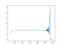
estimates for calculating $$e$$ with $$n$$ between 1 and $$1*10^{17}$$
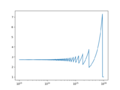
$$n$$ between $$10^{13}$$ and $$10^{16}$$ showing region when roundoff causes problems


Lecture 13 - 10/9 - Iterative Methods for Maps and Accumulations
- Taylor series fundamentals
- Maclaurin series approximation for exponential uses Chapra 4.2 to compute terms in an infinite sum.
- so
- Newton Method for finding square roots uses Chapra 4.2 to iteratively solve using a mathematical map. To find \(y\) where \(y=\sqrt{x}\):
\( \begin{align} y_{init}&=1\\ y_{new}&=\frac{y_{old}+\frac{x}{y_{old}}}{2} \end{align} \)
Lecture 14 - 10/13 - Logical Masks
- Basics of Python:Logical Masks
Lecture 15 - 10/15 - Monte Carlo Methods
- From Wikipedia: Monte Carlo method
- Poker hands and probabilities
Lecture 16 - 10/23 - Roots
- Python:Finding roots
- SciPy references (all from Optimization and root finding):
- scipy.optimize.brentq - closed method root finding
Lecture 17 - 10/27 - More Roots
- Roots continued
Lecture 18 - 10/30 - Optimization
- Python:Extrema
- SciPy references (all from Optimization and root finding):
- scipy.optimize.fmin - unbounded minimization
- scipy.optimize.fminbound - bounded minimization
Lecture 19 - 11/3 - Complex Number intro; Newton Fractals
Lecture 20 - 11/6 - Basic Linear Algebra
- 1D arrays are neither rows nor columns - they are 1D!
- 2D arrays have...two dimensions, one of which might be 1
- Python does mathematical operations differently for 1 and 2-D arrays
- Dot products as heart of matrix multiplication
- Inner dimensions must match; outer dimensions equal dimensions of result
- To multiply matrices A and B ($$C=A\times B$$ in math or
C=A@Bin Python) using matrix multiplication, the number of columns of A must match the number of rows of B; the results will have the same number of rows as A and the same number of columns as B. Order is important - Matrix multiplication (by hand)
- Matrix multiplication (using @ in Python)
- Reformatting linear algebra expressions as matrix equations
- Calculating determinants and inverses
- Determinants of matrices and the meaning when the determinant is 0
- Shortcuts for determinants of 1x1, 2x2 and 3x3 matrices (see class notes for processes)
- $$\begin{align*} \mbox{det}([a])&=a\\ \mbox{det}\left(\begin{bmatrix}a&b\\c&d\end{bmatrix}\right)&=ad-bc\\ \mbox{det}\left(\begin{bmatrix}a&b&c\\d&e&f\\g&h&i\end{bmatrix}\right)&=aei+bfg+cdh-afh-bdi-ceg\\ \end{align*}$$
- Don't believe me? Ask Captain Matrix!
- Inverses of matrices:
- In class, specifically looked at inverses of 1x1 and 2x2 - all that is required for this semester!
- But generally, $$\mbox{inv}(A)=\frac{\mbox{cof}(A)^T}{\mbox{det}(A)}$$ where the superscript T means transpose...
- And $$\mbox{det}(A)=\sum_{i\mbox{ or }j=0}^{N-1}a_{ij}(-1)^{i+j}M_{ij}$$ for some $$j$$ or $$i$$...
- And $$M_{ij}$$ is a minor of $$A$$, specifically the determinant of the matrix that remains if you remove the $$i$$th row and $$j$$th column or, if $$A$$ is a 1x1 matrix, 1
- And $$\mbox{cof(A)}$$ is a matrix where the $$i,j$$ entry $$c_{ij}=(-1)^{i+j}M_{ij}$$
- And $$M_{ij}$$ is a minor of $$A$$, specifically the determinant of the matrix that remains if you remove the $$i$$th row and $$j$$th column or, if $$A$$ is a 1x1 matrix, 1
- And $$\mbox{det}(A)=\sum_{i\mbox{ or }j=0}^{N-1}a_{ij}(-1)^{i+j}M_{ij}$$ for some $$j$$ or $$i$$...
- But generally, $$\mbox{inv}(A)=\frac{\mbox{cof}(A)^T}{\mbox{det}(A)}$$ where the superscript T means transpose...
- Again - Good news - for this class, you need to know how to calculate inverses of 1x1 and 2x2 matrices only:
- In class, specifically looked at inverses of 1x1 and 2x2 - all that is required for this semester!
- $$ \begin{align} \mbox{inv}([a])&=\frac{1}{a}\\ \mbox{inv}\left(\begin{bmatrix}a&b\\c&d\end{bmatrix}\right)&=\frac{\begin{bmatrix}d &-b\\-c &a\end{bmatrix}}{ad-bc} \end{align}$$
Lecture 21 - 11/10 - Numerical Integration
- Newton Interpolating Polynomials
- Overview of integration
- Riemann sums
- Trapezoidal Rule
- Simpson's 1/3 and 3/8 Rules
Lecture 22 - 11/13 - Numerical Differentiation
- Newton Interpolating Polynomials
- Overview of differentiation
- 2pt forward first derivative
- Exception at first point
- 2 pt backward first derivative
- Exception at last point
- 3pt centered first derivative
- Exceptions at first and last points
- 3pt centered second derivative
- Exceptions at first and last points
- 2pt forward first derivative
Lecture 23 - 11/17 - Object-oriented Programming
- Defining a class
- Initialization
- Dunder functions
- Other functions
- Building a bank class
Lecture 24 - 11/20 - More Object-oriented Programming
- Complex Numbers
- Building a complex number class
Lecture 25 - 11/27 - Curve Fitting
== Lecture 26 - 12/1 - Curve Fitting; Initial Value Problems
- General discussion of what a derivative is
- General discussion of what a differential equation is
Lecture 27 - 12/4 - More Initial Value Problems
- Euler-Cauchy program
- solve_ivp program
- Python:Ordinary Differential Equations
Lecture 28 - 12/8 - Demos
- Bouncing ball showing solve_ivp stop/restart conditions
- AI samples (identifying iris and wheat; visualizing histograms of characteristics)