ECE 280/Imaging Lab 1
This page serves as a supplement to the first Digital Image Processing Lab for ECE 280.
Contents
- 1 Corrections / Clarifications to the Handout
- 2 Running MATLAB
- 3 Image Processing Toolbox
- 4 Links
- 5 Examples
- 5.1 Example 1: Black & White Images
- 5.2 Example 2: Simple Grayscale Images
- 5.3 Example 3: Less Simple Grayscale Images
- 5.4 Example 4: Building an Image
- 5.5 Example 5: Exploring Colors
- 5.6 Example 6: 1D Convolution
- 5.7 Example 7: 1D Convolution Using 'same'
- 5.8 Example 8: 10x10 Blurring
- 5.9 Example 9: Make No Assumptions
- 5.10 Example 10: Basic Edge Detection and Display
- 5.11 Example 11: Chips!
- 5.12 Example 12: Chip Edges!
- 6 Exercise Starter Codes
Corrections / Clarifications to the Handout
- You will need the Image Processing Toolbox; if you do not have it, there is information below on how to install it.
Running MATLAB
MATLAB can be run remotely on the Duke Linux system, but it will generally be more convenient for you to install it on your own computer. All the documentation for this lab was written using MATLAB R2020a and tested with MATLAB R2021a. It is likely that MATLAB R2020b will also work. Previous versions of MATLAB have not been tested.
- Note: Evelyn (a previous Head TA) discovered that at least MATLAB 2018a uses 64 levels instead of 256 levels by default. If you are using an earlier version of MATLAB, when you create a colormap, you may need to write
colormap gray(256)instead of justcolormap grayin examples 2 and 8 and exercise 7 specifically.
Installing MATLAB
MATLAB is free for Duke students. Follow the instructions in the Installation section of the EGRWiki page on MATLAB. Be sure to select the appropriate PRODUCTS when asked.
Adding the Image Processing Toolbox
If you installed MATLAB on your own computer but do not have the Image Processing Toolbox:
- Go to the HOME tab in MATLAB
- Find and click on "Add-Ons"
- Search for Image Processing
- Click on the link for the Image Processing Toolbox
- Sign in to install if need be
- Install
Image Processing Toolbox
For this lab, there are a few commands you will need to learn (or remember):
imread('filename.ext')will load an image into MATLAB. Depending on the image type, the return from this function may be a matrix of binary numbers (black and white images), an array of integers between 0 and 255 (grayscale images), or a three-layer matrix of integers between 0 and 255 (color images).image(matrix)will display the contents of a matrix as viewed from above.- By default, the
imagecommand for a 1-layer matrix will assign colors based on a colormap that spans values from 0 to 255. Anything outside of that range will be clipped. - There are ways to change that, but you will not need to for this lab
- The
imagecommand for a 3-layer matrix will assign colors based on the first layer being the red component, the second layer being the green component, and the third layer being the blue component.- If the matrix is made up of floating-point numbers,
imageexpects those numbers to be in the range [0, 1] - If the matrix is made up of unsigned integers,
imageexpects those numbers to be in the range [0, 255] - If the matrix is made up of signed integers,
imageexpects those numbers to be in the range [-128, 127]
- If the matrix is made up of floating-point numbers,
- By default, the
imagesc(matrix)for a one layer matrix will display the contents of a matrix as viewed from above and will also map the minimum value to "color 0" and the maximum value to "color 255"; for a three-layer matrix it will work just likeimageimagesc(matrix, [c_low c_high)for a one layer matrix will display the contents of a matrix as viewed from above and will also map the colorsc_lowand below to "color 0" and colorsc_highand above to "color 255"; the colors in between will be linearly mapped to the colormap.colorbarwill add a...colorbar to the right of an image to show the numerical values and colors associated with them. This is only useful for a one-layer image.colormap MAPwill assign a particular colormap. For this assignment, the most useful one is gray for grayscale images.axis equalwill tell MATLAB to display an item such that each direction has the same scale. For the imaging commands, this is useful in that it will make each pixel a square regardless of the shape of the figure window, thus preserving the geometry of an image.
Links
- 2D Convolution link for 6.1: https://www.songho.ca/dsp/convolution/convolution2d_example.html
- Kernel link for Exercise 7: https://en.wikipedia.org/wiki/Kernel_(image_processing)
- Test Card for Exercise 8: https://en.wikipedia.org/wiki/Test_card
Examples
The following sections will contain both the example programs given in the lab as well as the image or images they produce. You should still type these into your own version of MATLAB to make sure you are getting the same answers. These are provided so you can compare what you get with what we think you should get.
Example 1: Black & White Images

a = [ 1 0 1 0 0; ...
      1 0 1 0 1; ...
      1 1 1 0 0; ...
      1 0 1 0 1; ...
      1 0 1 0 1 ];
figure(1); clf
imagesc(a)
colormap gray; colorbar
Example 2: Simple Grayscale Images

b = 0:255;
figure(1); clf
image(b)
colormap gray; colorbar
Example 3: Less Simple Grayscale Images

[x, y] = meshgrid(linspace(0, 2*pi, 201));
z = cos(x).*cos(2*y);
figure(1); clf
imagesc(z)
axis equal; colormap gray; colorbar
Notice how the use of axis equal made the image look like a square since it is 201x201 but also caused the display to be filled with whitespace as a result of the figure size versus the image size.
Example 4: Building an Image

rad = 100;
del = 10;
[x, y] = meshgrid((-3*rad-del):(3*rad+del));
[rows, cols] = size(x);
dist = @(x, y, xc, yc) sqrt((x-xc).^2+(y-yc).^2);
venn_img = zeros(rows, cols, 3);
venn_img(:,:,1) = (dist(x, y, rad.*cos(0), rad.*sin(0)) < 2*rad);
venn_img(:,:,2) = (dist(x, y, rad.*cos(2*pi/3), rad.*sin(2*pi/3)) < 2*rad);
venn_img(:,:,3) = (dist(x, y, rad.*cos(4*pi/3), rad.*sin(4*pi/3)) < 2*rad);
figure(1); clf
image(venn_img)
axis equal
Example 5: Exploring Colors

[x, y] = meshgrid(linspace(0, 1, 256));
other = 0.5;
palette = zeros(256, 256, 3);
palette(:,:,1) = x;
palette(:,:,2) = y;
palette(:,:,3) = other;
figure(1); clf
imagesc(palette)
axis equal
Example 6: 1D Convolution
x = [1, 2, 4, 8, 7, 5, 1]
h = [1, -1]
y = conv(x, h)
x =

     1     2     4     8     7     5     1


h =

     1    -1


y =

     1     1     2     4    -1    -2    -4    -1
Example 7: 1D Convolution Using 'same'
x = [1, 2, 4, 8, 7, 5, 1]
h = [1, -1]
y = conv(x, h, 'same')
x =

     1     2     4     8     7     5     1


h =

     1    -1


y =

     1     2     4    -1    -2    -4    -1
Example 8: 10x10 Blurring


x = imread('coins.png');
h = ones(10, 10)/10^2;
y = conv2(x, h, 'same');
figure(1); clf
image(x)
axis equal; colormap gray; colorbar
title('Original')
figure(2); clf
image(y)
axis equal; colormap gray; colorbar
title('10x10 Blur')
Example 9: Make No Assumptions
x = [1, 2, 4, 8, 7, 5, 1]
h = [1, -1]
y = conv(x, h, 'valid')
x =

     1     2     4     8     7     5     1


h =

     1    -1


y =

     1     2     4    -1    -2    -4
Example 10: Basic Edge Detection and Display
[x, y] = meshgrid(linspace(-1, 1, 200));
z1 = (.7<sqrt(x.^2+y.^2)) & (sqrt(x.^2+y.^2)<.9);
z2 = (.3<sqrt(x.^2+y.^2)) & (sqrt(x.^2+y.^2)<.5);
zimg = 100*z1+200*z2;
figure(1); clf
image(zimg);
axis equal; colormap gray; colorbar; title('Original')

hx = [1 -1; 1 -1];
edgex = conv2(zimg, hx, 'valid');
figure(2); clf
imagesc(edgex, [-512, 512]);
axis equal; colormap gray; colorbar; title('Vertical Edges')

hy = hx';
edgey = conv2(zimg, hy, 'valid');
figure(3); clf
imagesc(edgey, [-512, 512]);
axis equal; colormap gray; colorbar; title('Horizontal Edges')

edges = sqrt(edgex.^2 + edgey.^2);
figure(4); clf
imagesc(edges);
axis equal; colormap gray; colorbar; title('Edges')

Original
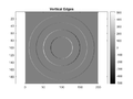
Vertical Edges

Horizontal Edges

Edges


Example 11: Chips!
clear
img = imread('coloredChips.png');
figure(1); clf
title('Original')
image(img); axis equal
vals = (0:255)'/255;
names = {'Red', 'Green', 'Blue'}
for k = 1:3
    figure(k+1); clf
    image(img(:,:,k)); axis equal
    colormap gray; colorbar
    title(names{k}+" as Gray")
    figure(k+4)
    image(img(:,:,k)); axis equal
    cmap = zeros(256, 3);
    cmap(:,k) = vals;
    colormap(cmap); colorbar
    title(names{k}+" as "+names{k})
end
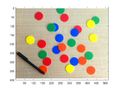
Original


Red as Gray

Green as Gray
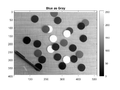
Blue as Gray


Red as Red

Green as Green

Blue as Blue


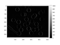
Example 12: Chip Edges!
clear
img = imread('coloredChips.png');
figure(1); clf
image(img); axis equal

h = [1 0 -1; 2 0 -2; 1 0 -1]
for k=1:3
    y(:,:,k) = conv2(img(:,:,k), h, 'valid');
    figure(1+k); clf
    imagesc(y(:,:,k), [-1020, 1020]);
    axis equal; colormap gray; colorbar
    figure(4+k); clf
    imagesc(abs(y(:,:,k)), [0, 1020]);
    axis equal; colormap gray; colorbar
end
%%
yx = (y+max(abs(y(:)))) / 2 / max(abs(y(:)));
figure(8); clf
image(yx); axis equal

yg = sqrt(y(:,:,1).^2 + y(:,:,2).^2 + y(:,:,3).^2);
ygs = abs(yg) / max(yg(:)) * 255;
figure(9); clf
image(ygs); colormap gray; axis equal

Original


Red Edges as Gray

Green Edges as Gray

Blue Edges as Gray


Absolute Red Edges as Gray
Absolute Green Edges as Gray

Absolute Blue Edges as Gray


Colorful Edges

Absolute Edges


Exercise Starter Codes
Exercise 3
tc = linspace(0, 1, 101);
xc = humps(tc);
td = linspace(0, 1, 11);
xd = humps(td);
figure(1); clf
plot(tc, xc, 'b-')
hold on
plot(td, xd, 'bo')
hold off
Exercise 4
tc = linspace(0, 1, 101);
xc = humps(tc);
deltatc = tc(2)-tc(1);
td = linspace(0, 1, 11);
xd = humps(td);
deltatd = td(2)-td(1);

figure(1); clf
plot(tc, xc, 'b-')
hold on
plot(td, xd, 'bo')
hold off
title('Values')

figure(2); clf
twopointdiff = diff(xc)/deltatc;
twopointdiff(end+1)=twopointdiff(end);
plot(tc, twopointdiff, 'b-')
hold on
plot(tc(1:10:end), twopointdiff(1:10:end), 'bo')
hold off
title('Change Me')