Difference between revisions of "MATLAB:Plotting Surfaces"
| Line 58: | Line 58: | ||
and the graph is: | and the graph is: | ||
<center> | <center> | ||
| − | [[Image:SurfExp01.png]] | + | [[Image:SurfExp01.png|400px]] |
</center> | </center> | ||
| Line 77: | Line 77: | ||
and the plot is | and the plot is | ||
<center> | <center> | ||
| − | [[Image:SurfExp02.png]] | + | [[Image:SurfExp02.png|400px]] |
</center> | </center> | ||
| Line 93: | Line 93: | ||
and the plot is: | and the plot is: | ||
<center> | <center> | ||
| − | [[Image:SurfExp03.png]] | + | [[Image:SurfExp03.png|400px]] |
</center> | </center> | ||
| Line 115: | Line 115: | ||
MinDistance = | MinDistance = | ||
0.0782 | 0.0782 | ||
| − | |||
MaxDistance = | MaxDistance = | ||
2.7803 | 2.7803 | ||
| − | |||
XatMin = | XatMin = | ||
-0.9474 | -0.9474 | ||
| − | |||
YatMin = | YatMin = | ||
-0.4421 | -0.4421 | ||
| − | |||
XatMax = | XatMax = | ||
1.2000 | 1.2000 | ||
| − | |||
YatMax = | YatMax = | ||
1.2000 | 1.2000 | ||
</source> | </source> | ||
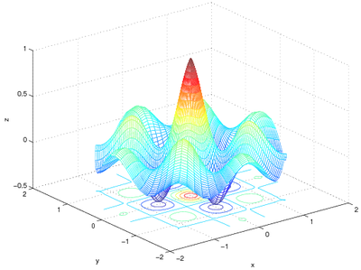
| − | If there are multiple maxima or minima, the | + | If there are multiple maxima or minima, the <code>find</code> command will |
| − | report them all | + | report them all. For example, with the following code, |
| − | + | <source lang="matlab"> | |
| + | [x, y] = meshgrid(linspace(-1, 1, 31)); | ||
z2 = exp(-sqrt(x.^2+y.^2)).*cos(4*x).*cos(4*y); | z2 = exp(-sqrt(x.^2+y.^2)).*cos(4*x).*cos(4*y); | ||
mesh(x, y, z2); | mesh(x, y, z2); | ||
| Line 147: | Line 143: | ||
XatMax = x(find(z2 == MaxVal)) | XatMax = x(find(z2 == MaxVal)) | ||
YatMax = y(find(z2 == MaxVal)) | YatMax = y(find(z2 == MaxVal)) | ||
| − | + | </source> | |
| − | + | which gives a graph of: | |
| − | + | <center> | |
| − | + | [[Image:SurfExp04.png|400px]] | |
| + | </center> | ||
| + | the matrix <code>z2</code> has four entries with the same minimum value and one with the maximum value: | ||
| + | <source lang="text"> | ||
| + | MinVal = | ||
| + | -0.4699 | ||
| − | |||
| − | |||
| − | |||
| − | |||
| − | |||
| − | |||
MaxVal = | MaxVal = | ||
| − | + | 1 | |
| + | |||
XatMin = | XatMin = | ||
| − | -0. | + | -0.7333 |
| − | + | 0 | |
| − | + | 0 | |
| − | 0. | + | 0.7333 |
| + | |||
YatMin = | YatMin = | ||
| − | + | 0 | |
| − | -0. | + | -0.7333 |
| − | 0. | + | 0.7333 |
| − | + | 0 | |
| + | |||
XatMax = | XatMax = | ||
| − | + | 0 | |
| + | |||
YatMax = | YatMax = | ||
| − | + | 0 | |
| − | + | </source> | |
| − | |||
| − | As seen in | + | == Higher Refinement == |
| + | As seen in creating line plots [[MATLAB:Plotting#Using_Different_Scales| using different scales]], you may want to use a more highly-refined | ||
grid to locate maxima and minima with greater precision. This may | grid to locate maxima and minima with greater precision. This may | ||
include reducing the overall domain of the function as well as | include reducing the overall domain of the function as well as | ||
| − | including more points. For example, the | + | including more points. For example, the changing the grid to have 1001 points in either direction makes for a more refined grid. The code below demonstrates how to increase the |
| − | |||
| − | |||
| − | makes for a more refined grid | ||
| − | |||
refinement: | refinement: | ||
| − | + | <source lang="matlab"> | |
| − | [xp, yp] = meshgrid(linspace(-1, 1, | + | [xp, yp] = meshgrid(linspace(-1.2, 1.2, 1001)); |
z2p = exp(-sqrt(xp.^2+yp.^2)).*cos(4*xp).*cos(4*yp); | z2p = exp(-sqrt(xp.^2+yp.^2)).*cos(4*xp).*cos(4*yp); | ||
MinValp = min(min(z2p)) | MinValp = min(min(z2p)) | ||
| Line 195: | Line 190: | ||
XatMaxp = xp(find(z2p == MaxValp)) | XatMaxp = xp(find(z2p == MaxValp)) | ||
YatMaxp = yp(find(z2p == MaxValp)) | YatMaxp = yp(find(z2p == MaxValp)) | ||
| − | + | </source> | |
The results obtained are: | The results obtained are: | ||
| − | + | <source lang="text"> | |
MinValp = | MinValp = | ||
-0.4703 | -0.4703 | ||
| + | |||
MaxValp = | MaxValp = | ||
1 | 1 | ||
| + | |||
XatMinp = | XatMinp = | ||
| − | -0. | + | -0.7248 |
0 | 0 | ||
0 | 0 | ||
| − | 0. | + | 0.7248 |
| + | |||
YatMinp = | YatMinp = | ||
0 | 0 | ||
| − | -0. | + | -0.7248 |
| − | 0. | + | 0.7248 |
0 | 0 | ||
| + | |||
XatMaxp = | XatMaxp = | ||
0 | 0 | ||
| + | |||
YatMaxp = | YatMaxp = | ||
0 | 0 | ||
| − | + | </source> | |
| − | Note that | + | Note that ''graphing'' the more refined points would be a bad idea - |
| − | there are now over | + | there are now over one million nodes and MATLAB will have a hard time |
rendering such a surface. | rendering such a surface. | ||
| − | \ | + | |
| + | == Using Other Coordinate Systems == | ||
| + | The plotting commands such as <code>mesh</code> and <code>surf</code> generate surfaces based on matrices of x, y, and z coordinates, respectively, but you can also use other coordinate systems to calculate where the points go. As an example, the surface above could be plotted on a circular domain using polar coordinates. To do that, ''r'' and <math>\theta</math> coordinates could be generated using meshgrid and the appropriate x, y, and z values could be obtained by noting that <math>x=r\cos(\theta)</math> and <math>y=r\sin(\theta)</math>. z can then be calculated from any combination of x, y, r, and <math>\theta</math>: | ||
| + | <source lang="matlab"> | ||
| + | [r, theta] = meshgrid(... | ||
| + | linspace(0, 1.7, 60), ... | ||
| + | linspace(0, 2*pi, 73)); | ||
| + | x = r.*cos(theta); | ||
| + | y = r.*sin(theta); | ||
| + | z = exp(-r).*cos(4*x).*cos(4*y); | ||
| + | mesh(x, y, z); | ||
| + | xlabel('x'); | ||
| + | ylabel('y'); | ||
| + | zlabel('z'); | ||
| + | </source> | ||
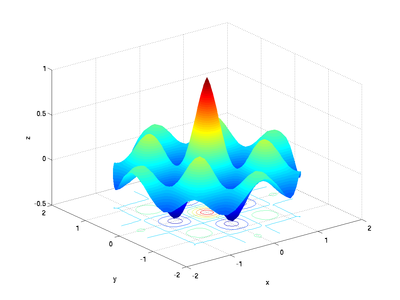
| + | produces: | ||
| + | <center> | ||
| + | [[Image:SurfExp06a.png|400px]] | ||
| + | </center> | ||
| + | though in this case, an interpolated surface plot might look better: | ||
| + | <source lang="matlab"> | ||
| + | surf(x, y, z); | ||
| + | shading interp | ||
| + | xlabel('x'); | ||
| + | ylabel('y'); | ||
| + | zlabel('z'); | ||
| + | </source> | ||
| + | <center> | ||
| + | [[Image:SurfExp06b.png|400px]] | ||
| + | </center> | ||
| + | |||
| + | |||
| + | == Questions == | ||
| + | {{Questions}} | ||
| + | |||
| + | == External Links == | ||
| + | |||
| + | == References == | ||
| + | <references /> | ||
Revision as of 19:13, 20 September 2008
There are many problems in engineering that require examining a 2-D domain. For example, if you want to determine the distance from a specific point on a flat surface to any other flat surface, you need to think about both the x and y coordinate. There are various other functions that need x and y coordinates.
Contents
The meshgrid Command
The meshgrid command is specifically used to create matrices that will represent x and y coordinates. For example, note the output to the following MATLAB command:
[x, y] = meshgrid(-2:1:2, -1:.25:1)
x =

    -2    -1     0     1     2
    -2    -1     0     1     2
    -2    -1     0     1     2
    -2    -1     0     1     2
    -2    -1     0     1     2
    -2    -1     0     1     2
    -2    -1     0     1     2
    -2    -1     0     1     2
    -2    -1     0     1     2

y =

   -1.0000   -1.0000   -1.0000   -1.0000   -1.0000
   -0.7500   -0.7500   -0.7500   -0.7500   -0.7500
   -0.5000   -0.5000   -0.5000   -0.5000   -0.5000
   -0.2500   -0.2500   -0.2500   -0.2500   -0.2500
         0         0         0         0         0
    0.2500    0.2500    0.2500    0.2500    0.2500
    0.5000    0.5000    0.5000    0.5000    0.5000
    0.7500    0.7500    0.7500    0.7500    0.7500
    1.0000    1.0000    1.0000    1.0000    1.0000
The first argument gives the range that the first output variable
should include, and the second argument gives the range that the
second output variable should include. Note that the first output
variable x basically gives an x coordinate and the second output
variable y gives a y coordinate. This is useful if you want to
plot a function in 2-D.
Examples Using 2 Independent Variables
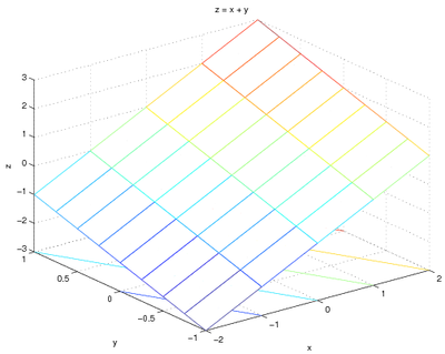
For example, to plot z=x+y over the ranges of x
and y specified above - the code would be:
z = x + y;
mesh(x, y, z);
xlabel('x');
ylabel('y');
zlabel('z');
title('z = x + y');
and the graph is:

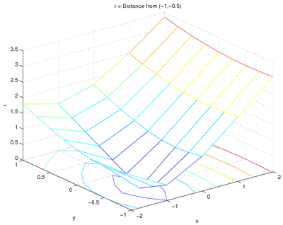
To find the distance r from a particular point, say (-1,-0.5), you just need
to change the function.  Since the distance between two points \((x, y)\) and \((x_0, y_0)\) is given by
\(
r=\sqrt{(x-x_0)^2+(y-y_0)^2}
\)
the code could be:
r = sqrt( (x-(-1)).^2 + (y-(-0.5)).^2 );
mesh(x, y, r);
xlabel('x');
ylabel('y');
zlabel('r');
title('r = Distance from (-1,-0.5)');
and the plot is

Examples Using Refined Grids
You can also use a finer grid to make a better-looking plot:
\begin{lstlisting}[frame=single]
[x, y] = meshgrid(linspace(-1.2, 1.2, 20));
r = sqrt( (x-(-1)).^2 + (y-(-0.5)).^2 );
mesh(x, y, r);
xlabel('x');
ylabel('y');
zlabel('r');
title('r = Distance from (-1,-0.5)');
</source>
and the plot is:
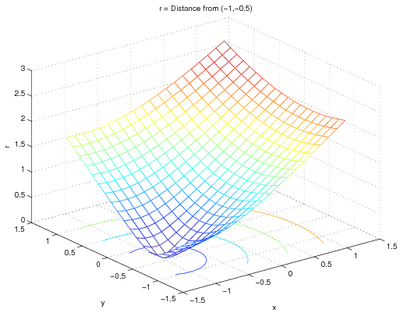

Note that the meshgrid,/code> command was given only one
argument - in that case, the range of x and y will be the same.
Finding Minima and Maxima in 2-D
You can also use these 2-D structures to find minima and maxima.  For
example, given the grid in the code directly above, you can find the
minimum and maximum distances and where they occur:
MinDistance = min(r(:))
MaxDistance = max(r(:))
XatMin = x(find(r == MinDistance))
YatMin = y(find(r == MinDistance))
XatMax = x(find(r == MaxDistance))
YatMax = y(find(r == MaxDistance))
MinDistance =
    0.0782
MaxDistance =
    2.7803
XatMin =
   -0.9474
YatMin =
   -0.4421
XatMax =
    1.2000
YatMax =
    1.2000
If there are multiple maxima or minima, the find command will
report them all.  For example, with the following code,
    [x, y] = meshgrid(linspace(-1, 1, 31));
z2 = exp(-sqrt(x.^2+y.^2)).*cos(4*x).*cos(4*y);
mesh(x, y, z2);
xlabel('x');
ylabel('y');
zlabel('z');
title('z = e^{-(x^2+y^2)^{0.5}} cos(4x) cos(4y)');
MinVal = min(min(z2))
MaxVal = max(max(z2))
XatMin = x(find(z2 == MinVal))
YatMin = y(find(z2 == MinVal))
XatMax = x(find(z2 == MaxVal))
YatMax = y(find(z2 == MaxVal))
which gives a graph of:
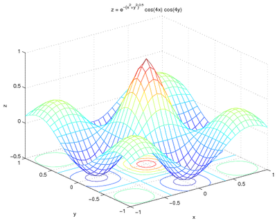

the matrix z2 has four entries with the same minimum value and one with the maximum value:
MinVal =
   -0.4699

MaxVal =
     1

XatMin =
   -0.7333
         0
         0
    0.7333

YatMin =
         0
   -0.7333
    0.7333
         0

XatMax =
     0

YatMax =
     0
Higher Refinement
As seen in creating line plots  using different scales, you may want to use a more highly-refined
grid to locate maxima and minima with greater precision.  This may
include reducing the overall domain of the function as well as
including more points.  For example, the changing the grid to have 1001 points in either direction  makes for a more refined grid.  The code below demonstrates how to increase the
refinement:
[xp, yp] = meshgrid(linspace(-1.2, 1.2, 1001));
z2p = exp(-sqrt(xp.^2+yp.^2)).*cos(4*xp).*cos(4*yp);
MinValp = min(min(z2p))
MaxValp = max(max(z2p))
XatMinp = xp(find(z2p == MinValp))
YatMinp = yp(find(z2p == MinValp))
XatMaxp = xp(find(z2p == MaxValp))
YatMaxp = yp(find(z2p == MaxValp))
The results obtained are:
MinValp =
   -0.4703

MaxValp =
     1

XatMinp =
   -0.7248
         0
         0
    0.7248

YatMinp =
         0
   -0.7248
    0.7248
         0

XatMaxp =
     0

YatMaxp =
     0
Note that graphing the more refined points would be a bad idea -
there are now over one million nodes and MATLAB will have a hard time
rendering such a surface.
Using Other Coordinate Systems
The plotting commands such as mesh and surf generate surfaces based on matrices of x, y, and z coordinates, respectively, but you can also use other coordinate systems to calculate where the points go. As an example, the surface above could be plotted on a circular domain using polar coordinates. To do that, r and \(\theta\) coordinates could be generated using meshgrid and the appropriate x, y, and z values could be obtained by noting that \(x=r\cos(\theta)\) and \(y=r\sin(\theta)\). z can then be calculated from any combination of x, y, r, and \(\theta\):
 [r, theta] = meshgrid(...
        linspace(0, 1.7, 60), ...
        linspace(0, 2*pi, 73));
    x = r.*cos(theta);
    y = r.*sin(theta);
    z = exp(-r).*cos(4*x).*cos(4*y);
    mesh(x, y, z);
    xlabel('x');
    ylabel('y');
    zlabel('z');
produces:

though in this case, an interpolated surface plot might look better:
surf(x, y, z);
shading interp
xlabel('x');
ylabel('y');
zlabel('z');

Questions
Post your questions by editing the discussion page of this article. Edit the page, then scroll to the bottom and add a question by putting in the characters *{{Q}}, followed by your question and finally your signature (with four tildes, i.e. ~~~~). Using the {{Q}} will automatically put the page in the category of pages with questions - other editors hoping to help out can then go to that category page to see where the questions are. See the page for Template:Q for details and examples.
External Links
References