SymPy/Differential Equations/RC Example

Description

The following page is adapted from Maple/Differential Equations/RC Example and will go through an example of using SymPy's ability to symbolically solve a differential equation - specifically to analyze a circuit that undergoes a change in source values. In this particular case, the independent source is given as a constant for all times before 0 sec, at which time it changes to a non-constant source. The source is connected to a network containing both resistors and a capacitor. While there are several ways to put all this work together in Python, the following will provide a flexible framework for solving the equations and using substitution to determine a numerical list of initial conditions, substituting element values into the differential equations and putting them into a list, solving the differential equations, and finally plotting the results.

Note: at the moment, SymPy's dsolve command works pretty well for up to two coupled ODEs but starts having issues once a third equation is in the mix. Unlike Maple, which has the option to use Laplace techniques with its dsolve command, SymPy does not. Roundoff and other errors creep in, causing the solution to fail to match the initial conditions. For higher-order systems, at the moment, a numerical solver such as solve_ivp might be required (which also requires breaking the system down into a series of first-order differential equations).

Circuit

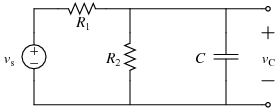
For this demonstration code, the following circuit is used:

where \(R_1\)=20 k\(\Omega\), \(R_2\)=30 k\(\Omega\), \(C\)=50 \(\mu\)F, and \(v_s(t)\) changes from 5 V to 10 cos(8\(t\)) V when \(t=0\) s.

DC Steady-State Analysis

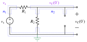
Assuming the circuit has been in place for a "long time" before \(t\)=0 sec, and given the topology of the circuit and the fact that the independent source is a constant for all times before 0 sec, you can use the DC steady-state equivalent for the circuit at \(t=0^-\) sec:

Using KCL at the top right node gives:

\( \frac{v_C(0^-)-v_S}{R_1}+ \frac{v_C(0^-)}{R_2}=0\! \)

which can be solved to find the capacitor voltage at the time just before the source \(v_S(t)\) changes.

Model Equations for t>0

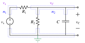
In general, after \(t\)=0 sec you can label the circuit as:

Using KCL at the top right node again gives:

\( \frac{v_C(t)-v_S(t)}{R_1}+ \frac{v_C(t)}{R_2}+C\frac{dv_C(t)}{dt}=0\! \)

Code

Now that the equations for DC steady state and for the differential model are known, you can write a Python script to solve for everything.

Initialization

You will need to import sympy to use symbolic calculations. You will also need numpy and matplotlib.pyplot to make a graph.

import sympy as sym
import numpy as np
import matplotlib.pyplot as plt

Because you are solving systems of differential equations, the same helper functions that were used to solve simultaneous equations will be useful. Given that, your script should import the helper functions from sym_helper.py; you can do this with:

# Import the helper functions
try:
  from sym_helper import *
except: # Get sym_helper.py from GitHub
  import requests
  url = 'https://tinyurl.com/mrgdemos/SymPy_Files/sym_helper.py'
  open('sym_helper.py', 'w').write(requests.get(url).text)
  from sym_helper import *

Finally, you will want the script to use $$\LaTeX$$ to display your equations if possible:

# Use LaTeX if possible
sym.init_printing(use_latex=True)

Declaring Variables and Functions

Next you should tell SymPy what your variables are. You will also need to declare the functions' that you will be using later. For this example, the known values include the two resistors, the capacitor, the DC value of the source before time 0, and time. The functions you will want to declare include the (potentially non-constant) voltage of the source after time 0 and the voltage across the capacitor. You may also want to create a list of the known variables and a list of the values of those variables:

R1, R2, C, vsdc, t = sym.var('R1, R2, C, v_{s\,dc}, t')
vs = sym.Function("v_s")
vC = sym.Function("v_C")
knowns = R1, R2, C, vsdc, vs(t)
knownvals = [20000, 30000, 50e-6, 5, 10*sym.cos(8*t)]

Initial Conditions From Steady-State

While SymPy can solve some differential equations with symbolic initial conditions and coefficients, most of the time this will result in a very unwieldy and unhelpful representation. For this assignment, you will be providing SymPy with numerical values for the initial conditions. To do this, we are going to ask SymPy to solve the linear algebra problem that comes from the DC steady state and then we will substitute in numerical values. First, we will define a variable to be the initial condition of the capacitor voltage and will add it to a list of unknowns:

vC0 = vC(t).subs(t, 0)
unksSS = [vC0]

Next, we will write the conservation equation we have at DC steady-state and add it to a list of equations:

eqn1SS = (vC0-vsdc) / R1 + vC0 / R2
eqnsSS = [eqn1SS]

Finally, we can solve the equation and then substitute in numerical values:

solnSS = sym.solve(eqnsSS, unksSS)
solnSSnum = makesubs(solnSS, knowns, knownvals)

This results in solnSSnum being a dictionary with the initial value of $$v_C$$ defined in it, $$\{v_C(0):3\}$$

Differential Equations

Next we can set up and solve the differential equations. First, make a list of all the unknown functions for which you want to solve:

unks = [vC(t)]

You can now write the differential equations (using sym.Derivative(FUN, VAR) to represent the derivatives) and put them in a list:

eq1 = (vC(t)-vs(t))/R1 + vC(t)/R2 + C*sym.Derivative(vC(t), t)
eqns = [eq1]

While it is possible for SymPy to solve some systems purely symbolically, there are times where it is much easier for it to solve equations where the coefficients are numbers. To help with that, the sym_helper file has a command called makesubseqnlist(LIST, KNOWNVARLIST, KNOWNVALLIST) that will take a list of equations and substitute the given values in for the given variables. The code for makesubeqnlist is:

def makesubseqnlist(equations, vartosub, valtosub):
    sublist = list(zip(vartosub, valtosub))
    esub = []    
    for eqn in equations:
      esub.append(eqn.subs(sublist))
    return esub

and the code that will go in your script for this is:

neqns = makesubseqnlist(eqns, knowns, knownvals)

Now you can solve the differential equations using dsolve:

solnlist = sym.dsolve(neqns, unks, ics=solnSSnum)

Note: unlike solve, which creates a dictionary of solutions, dsolve creates a list. It turns out having a dictionary makes life much easier later, so sym_helper has a make_dict(LIST) command that will turn a list of equations into a dictionary. The code for make_dict is:

def makedict(sollist):
    d = {}
    for eqn in sollist:
        d[eqn.lhs] = eqn.rhs
    return d

and so the code you can add to your script is:

def makedict(sollist):
soln = makedict(solnlist)

Plotting

Plotting will require using lambdify to turn one or more functions into a lambda function and then setting up your plot. Here is the code for this example that does all those things (making a plot that runs from $$t$$=0 to 10 sec):

vCfun = sym.lambdify(t, soln[vC(t)])
fig = plt.figure(num=1, clear=True)
ax = fig.add_subplot(1, 1, 1)
tn = np.linspace(0, 10, 1000)
ax.plot(tn, vCfun(tn))

Complete Example

For the Spring 2023 semester, students in EGR 224 get the code by going to the Google Colab version of it. This notebook includes several more comments than are listed above and has multiple instances where it displays intermediate results.