MATLAB:Polynomial Interpolation vs. Fit

Introduction

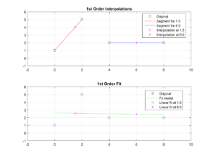
Polynomial interpolation is different from polynomial fitting. Polynomial fitting seeks to take a single polynomial - generally of a low order - and finds the coefficients which gets the polynomial collectively as close to all the points as possible, but which may not actually hit any of the points.

Polynomial interpolation will always be of an order one less than the number of points used; it will always go through the basis points you use to create the interpolation. For instance, a first order polynomial interpolation will always use the straight line between the two closes points in the data set. A second order polynomial interpolation will always use the quadratic that interpolates among the nearest three points -- depending on spacing, there may be two different but equally valid sets of points to you.

Example

The code and graph below will show the differences between the code for and meaning of polynomial interpolation (top) and fitting (bottom). In this case, the goal is to find two different values - one at x=1.5 and one at x=6.

clear; format short e
x = [0 2 4 8]
y = [1 5 2 2]

figure(1); clf
subplot(2, 1, 1)
%% Plot original data
plot(x, y, 'ko')
hold on
%% Plot segment of closest basis points
plot(x(1:2), y(1:2), 'r-')
plot(x(3:4), y(3:4), 'b-')
%% Calculate and plot interpolated values
yInterp1p5 = polyval(polyfit(x(1:2),y(1:2),1),1.5)
yInterp6p0 = polyval(polyfit(x(3:4),y(3:4),1),6)
plot(1.5, yInterp1p5, 'ms', 6, yInterp6p0, 'm*')
%% Extra
legend('Original', 'Segment for 1.5', 'Segment for 6.0', ...
    'Interpolation at 1.5', 'Interpolation at 6.0', ...
    'Location', 'Best')
grid on
title('1st Order Interpolations')
axis([-2 10 -1 6])

subplot(2, 1, 2)
%% Plot original data
plot(x, y, 'ko')
%% Calculate model across entire domain and plot
xm = linspace(x(1), x(end), 100);
ym = polyval(polyfit(x, y, 1), xm);
hold on
plot(xm, ym, 'g-')
% Calculate and plot estimate using fit
yFit1p5 = polyval(polyfit(x,y,1),1.5)
yFit6p0 = polyval(polyfit(x,y,1),6)
plot(1.5, yFit1p5, 'ms', 6, yFit6p0, 'm*')
%% Extra
legend('Original', 'Fit model', ...
    'Linear fit at 1.5', 'Linear fit at 6.0', ...
    'Location', 'Best')
grid on
title('1st Order Fit')
axis([-2 10 -1 6])

print -dpng FitVersusInterp