Difference between revisions of "Maple/Plotting"
m |
|||
| Line 49: | Line 49: | ||
for plot as well as a help file for plot options. The main ones to | for plot as well as a help file for plot options. The main ones to | ||
use here will be the <code>labels</code>, <code>labeldirections</code>, <code>title</code>, | use here will be the <code>labels</code>, <code>labeldirections</code>, <code>title</code>, | ||
| − | + | <code>legend</code>, and <code>linestyle</code>. Options | |
go after the independent argument and are separated by commas. For | go after the independent argument and are separated by commas. For | ||
example, a more complete version of the trig plot above might be: | example, a more complete version of the trig plot above might be: | ||
Revision as of 20:09, 12 February 2012
Maple has several built in commands to make plots. This page will show you how to use the {\tt plot} command.
Basics
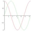
The command generally takes at least two arguments - an array of items to plot and a statement about the independent variable and its values. For example, to plot cos and sin over one period, you could type:
plot([cos(t), sin(t)], t = 0 .. 2*Pi)
If you have a variable that has several unknowns, you can use the
subs command to make substitutions for all but the independent
variable of the plot. For example, given some function \(f\):
which can be defined in Maple using the code:
f:=exp(-t)*cos(omega*t-k*x)
and assuming \(\omega\) is known to be 5 rad/s and \(k\) is 3 rad/m, you could make a plot of \(f\) at \(t=10\) s over the course of a 2 m section:
FVals:= omega=5, k=3;
plot(subs(FVals, t=10, f), x=0..2)
With the same equation, then, you could make a plot of \(f\) at the 6 m mark for times between 0 and 4 just by switching the variables around a bit:
FVals:= omega=5, k=3;
plot(subs(FVals, x=6, f), t=0..4)
Simple plotting example
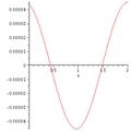
Plot of \(e^{-10}\cos(50-3x)\)
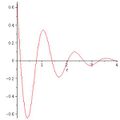
Plot of \(e^{-t}\cos(5t-12)\)


Plot Options

There are several plot options, which are described in the help file
for plot as well as a help file for plot options. The main ones to
use here will be the labels, labeldirections, title,
legend, and linestyle. Options
go after the independent argument and are separated by commas. For
example, a more complete version of the trig plot above might be:
plot([cos(t), sin(t)], t = 0 .. 2*Pi,
labels = ["Time (t)", "Voltage (V)"],
labeldirections = [horizontal, vertical],
title = "Cosine and Sin (mrg)",
legend = ["cos(t)", "sin(t)"],
linestyle=[4,2])
Note - using Shift-Enter will go to a new line.
Plotting Functions with Vestigial Imaginary Parts
Oftentimes, solving differential equations or inverse Laplace transforms will yield small roundoff errors that cause a function which should be purely real to have a vestigial imaginary component. To eliminate this - and thus make it possible to see the plot - use Maple's map command to apply the Re command to your function. For example, if MySoln contains a set of solutions for variables a(t), b(t), and c(t), and those variables have leftover imaginary parts, you could use:
plot(map(Re, subs(MySoln[], [a(t), b(t), c(t)])), t=0..1)
to plot just the real parts. If a plot line seems to "disappear" over the domain of the plot, the usual cause is the extra imaginary part that needs to be eliminated.