MATLAB:Plotting Surfaces
There are many problems in engineering that require examining a 2-D domain. For example, if you want to determine the distance from a specific point on a flat surface to any other flat surface, you need to think about both the x and y coordinate. There are various other functions that need x and y coordinates.
The meshgrid Command
The meshgrid command is specifically used to create matrices that will represent x and y coordinates. For example, note the output to the following MATLAB command:
[x, y] = meshgrid(-2:1:2, -1:.25:1)
x =

    -2    -1     0     1     2
    -2    -1     0     1     2
    -2    -1     0     1     2
    -2    -1     0     1     2
    -2    -1     0     1     2
    -2    -1     0     1     2
    -2    -1     0     1     2
    -2    -1     0     1     2
    -2    -1     0     1     2

y =

   -1.0000   -1.0000   -1.0000   -1.0000   -1.0000
   -0.7500   -0.7500   -0.7500   -0.7500   -0.7500
   -0.5000   -0.5000   -0.5000   -0.5000   -0.5000
   -0.2500   -0.2500   -0.2500   -0.2500   -0.2500
         0         0         0         0         0
    0.2500    0.2500    0.2500    0.2500    0.2500
    0.5000    0.5000    0.5000    0.5000    0.5000
    0.7500    0.7500    0.7500    0.7500    0.7500
    1.0000    1.0000    1.0000    1.0000    1.0000
The first argument gives the range that the first output variable
should include, and the second argument gives the range that the
second output variable should include. Note that the first output
variable x basically gives an x coordinate and the second output
variable y gives a y coordinate. This is useful if you want to
plot a function in 2-D.
Examples Using 2 Independent Variables
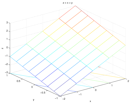
For example, to plot z=x+y over the ranges of x
and y specified above - the code would be:
z = x + y;
mesh(x, y, z);
xlabel('x');
ylabel('y');
zlabel('z');
title('z = x + y');
and the graph is:

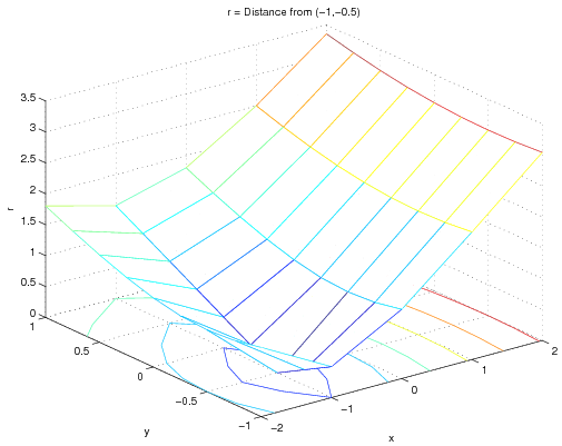
To find the distance r from a particular point, say (-1,-0.5), you just need
to change the function.  Since the distance between two points \((x, y)\) and \((x_0, y_0)\) is given by
\(
r=\sqrt{(x-x_0)^2+(y-y_0)^2}
\)
the code could be:
r = sqrt( (x-(-1)).^2 + (y-(-0.5)).^2 );
mesh(x, y, r);
xlabel('x');
ylabel('y');
zlabel('r');
title('r = Distance from (-1,-0.5)');
and the plot is

Examples Using Refined Grids
You can also use a finer grid to make a better-looking plot:
\begin{lstlisting}[frame=single]
[x, y] = meshgrid(linspace(-1.2, 1.2, 20));
r = sqrt( (x-(-1)).^2 + (y-(-0.5)).^2 );
mesh(x, y, r);
xlabel('x');
ylabel('y');
zlabel('r');
title('r = Distance from (-1,-0.5)');
</source>
and the plot is:
<center>
[[Image:SurfExp03.png]]
</center>

Note that the <code>meshgrid,/code> command was given only one
argument - in that case, the range of <code>x</code> and <code>y</code> will be the same.

=='"`UNIQ--h-3--QINU`"' Finding Minima and Maxima in 2-D ==
You can also use these 2-D structures to find minima and maxima.  For
example, given the grid in the code directly above, you can find the
minimum and maximum distances and where they occur:
'"`UNIQ--source-00000008-QINU`"'

'"`UNIQ--source-0000000A-QINU`"'

If there are multiple maxima or minima, the {\tt find} command will
report them all:
\begin{lstlisting}[frame=single]
z2 = exp(-sqrt(x.^2+y.^2)).*cos(4*x).*cos(4*y);
mesh(x, y, z2);
xlabel('x');
ylabel('y');
zlabel('z');
title('z = e^{-(x^2+y^2)^{0.5}} cos(4x) cos(4y)');
MinVal = min(min(z2))
MaxVal = max(max(z2))
XatMin = x(find(z2 == MinVal))
YatMin = y(find(z2 == MinVal))
XatMax = x(find(z2 == MaxVal))
YatMax = y(find(z2 == MaxVal))
\end{lstlisting}
\begin{center}
\epsfig{file=PROGRAMMING2/MeshPlot4.eps, width=3.7in}
\end{center}
\noindent
In this case, based on the grid, there are four minima and one
maximum, specifically:
\begin{lstlisting}[frame=LR]
MinVal =
   -0.4526
MaxVal =
    0.8877
XatMin =
   -0.6842
    0.0526
    0.0526
    0.6842
YatMin =
    0.0526
   -0.6842
    0.6842
    0.0526
XatMax =
    0.0526
YatMax =
    0.0526
\end{lstlisting}
\pagebreak
As seen in previous labs, you may want to use a more highly-refined
grid to locate maxima and minima with greater precision.  This may
include reducing the overall domain of the function as well as
including more points.  For example, the {\it true} maximum of the
function above should be at exactly (0, 0) and should have a value of
1.  Changing the grid to have 501 points in either direction both
makes for a more refined grid {\it and} makes sure that the grid
include the origin.  The code below demonstrates how to increase the
refinement:
\begin{lstlisting}[frame=single]
[xp, yp] = meshgrid(linspace(-1, 1, 501));
z2p = exp(-sqrt(xp.^2+yp.^2)).*cos(4*xp).*cos(4*yp);
MinValp = min(min(z2p))
MaxValp = max(max(z2p))
XatMinp = xp(find(z2p == MinValp))
YatMinp = yp(find(z2p == MinValp))
XatMaxp = xp(find(z2p == MaxValp))
YatMaxp = yp(find(z2p == MaxValp))
\end{lstlisting}
The results obtained are:
\begin{lstlisting}[frame=LR]
MinValp =
   -0.4703
MaxValp =
     1
XatMinp =
   -0.7240
         0
         0
    0.7240
YatMinp =
         0
   -0.7240
    0.7240
         0
XatMaxp =
     0
YatMaxp =
     0
\end{lstlisting}
Note that {\it graphing} the more refined points would be a bad idea -
there are now over 250,000 nodes and MATLAB will have a hard time
rendering such a surface.
\pagebreak